Drums libraries have been one of the most important developments in digital music production. We’re no longer restricted to the stock sounds that come with drum machines, allowing for more room to develop a unique sound. We’ve seen a surge in free drum kits on the web, and there’s an ever-growing list of digital audio workstations with which to use them.
As my own drum library has exploded in size (ok I’m a hoarder), it’s got me thinking of ways to take control and organize it better. One thing that has bugged me is the inconsistent naming of sound files:
- Abbreviations like
CR.wavfor a crash cymbal, that wouldn’t come up in a search - Different classification schemes, e.g.
Perc.wavfor ‘percussion’, instead of something more specific like rimshot - Labels I don’t agree with, or are just flat out wrong
It would help to have my own way of assigning drum sound labels, and in this post I will share several ways to achieve that with ML.
All code is open-source, so you can follow along and try this out yourself! You only need python and your own drum sounds.
What do drum sounds look like?
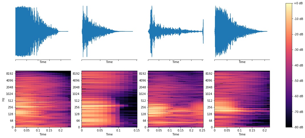
If you’ve ever worked with audio data you’re probably familiar with waveforms, which show the raw signals that might be sent to speakers for playback. Spectrograms are more insightful because they separate a signal into different frequency bands, allowing you to see the amount of energy up and down the spectrum. See examples of both below.
Snares
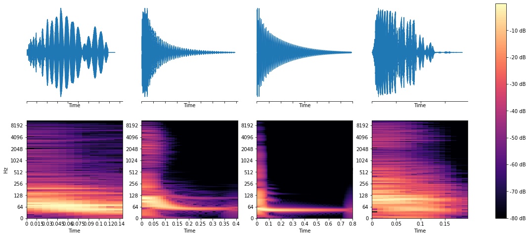
Kicks
Toms
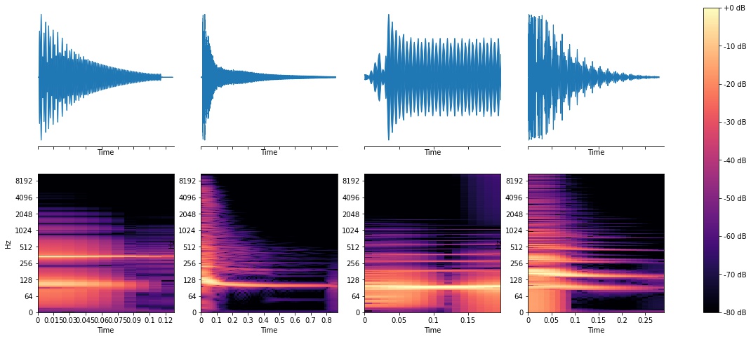
Plots above made with librosa, a great python library for audio processing.
You’ll notice some patterns, like how the snare waveforms look “fuzzier” and have energy up and down the spectrum. Kicks are obviously strongest in the lower frequencies (you can see spikes around 64 Hz), and toms look similar to kicks in ways but have spikes anywhere from 100Hz-500Hz. Now, lets see what ML can do.
A taxonomy
I needed a set of drum type classes. A few options came up in research, the simplest being bass drum, snare drum, hi-hat (used in this thesis and elsewhere). A limited set like that would make prediction easy, but it’s not as useful. The authors of one paper used a scheme closer to that of a standard rock kit: kick, snare, low tom, medium tom, high tom, open hi-hat, closed hi-hat, ride, crash. There’s even the General MIDI spec with dozens of percussive types – though, with that many classes it becomes hard to build up a dataset with enough of each.
I wanted to strike the right balance of taxonomy size, while also choosing classes more reflective of modern hip-hop and electronic drum kits found on the web. So, I made my own: hat, tom, ride [cymbal], open [hi-hat], kick, bongo [and conga], clap, snare, rim, snap, crash [cymbal], shaker
Building a clean dataset
Drum libraries are usually scattered across different folders, so given the top-level folder, it shouldn’t be hard to recursively walk and find all eligible sounds. I’m a fan of using pandas to explore data, so I initialized a DataFrame with one sound per row.
def read_drum_library(input_dir_path):
    logger.info(f'Searching for audio files found in {input_dir_path}')

    dataframe_rows = []
    for input_file in input_dir_path.glob('**/*.*'):
        absolute_path_name = input_file.resolve().as_posix()
        if not can_load_audio(absolute_path_name):
            continue

        properties = {
            'audio_path': absolute_path_name,
            'store_path': file_store_path.as_posix(),
            'file_stem': Path(absolute_path_name).stem.lower(),
            'start_time': 0.0,
            'end_time': np.NaN
        }
        # Tack on the original file duration (will have to load audio)
        audio = read_audio.load_raw_audio(absolute_path_name, fast=True)
        properties['orig_duration'] = len(audio) / float(read_audio.DEFAULT_SR)

        dataframe_rows.append(properties)

    return pandas.DataFrame(dataframe_rows)
I got rid of really quiet sounds by thresholding RMS, and also excluded those over 5 seconds.
I wanted to go even further in isolating single percussive hits, because I had noticed some loops with multiple hits that might throw off a model. I also wanted some consistency around how much silence appeared at the begging of sounds. My solution for both of these issues was to use librosa’s onset detection API. An onset is the moment that marks the beginning of a rise in energy of a sound. All I had to do is set the start time of each sound to just before the first onset, and the end time to just before any second onset.
One downside of the supervised deep learning techniques we’ll see later is that they require a lot of data. It’s easy to find tons of drum kits on the web, but what about labels? Fortunately, we can build up a dataset without manual annotations by just trusting the original filenames. They won’t be perfect, but they’ll be good enough to start.
DRUM_TYPES = ['hat', 'tom', 'ride', 'open', 'kick', 'bongo', 'clap', 'snare', 'rim', 'snap', 'crash', 'shaker']
drums_df = read_drum_library(drum_lib_path)
for drum_type_class in DRUM_TYPES:
    drum_sounds.loc[drum_sounds.file_stem.str.contains(drum_type_class), 'file_drum_type'] = drum_type_class
If you’re following along at home, you can run:
python preprocess.py --drum_lib_path ~/Music/drums
With that, my dataset looked like this:
> import pickle
> drums = pickle.load(open('data/interim/dataset.pkl', 'rb'))
> drums = drums[~drums.file_drum_type.isna()]   # Restrict to sounds with recognizable file labels
> drums.info()
Data columns (total 7 columns):
 #   Column          Non-Null Count     Dtype
---  ------          --------------     -----
 0   audio_path      11672 non-null     object
 1   store_path      11672 non-null     object
 2   file_stem       11672 non-null     object
 3   start_time      11672 non-null     float64
 4   end_time        818   non-null     float64
 5   orig_duration   11672 non-null     float64
 6   file_drum_type  11672 non-null     object
dtypes: float64(3), object(4)
memory usage: 1.2+ MB

> drums[['file_stem', 'start_time', 'end_time', 'file_drum_type']].sample(5)
   file_stem  start_time  end_time file_drum_type
15   openhat    0.000000       NaN           open
5     kick18    0.000000       NaN           kick
38   schat13    0.000000       NaN            hat
2    lakick9    0.000000       NaN           kick
19    kick8     0.022653  0.092494           kick

> drums.drum_type.value_counts()
snare     2952
kick      2845
hat       1805
tom       1371
clap      1048
rim        436
open       337
ride       263
crash      257
snap       110
bongo      101
shaker      98
As you can see, I had a pretty large class imbalance. This can be bad for model performance on the lesser represented classes. One way to help with this is over-sampling via something like imbalanced-learn or pyTorch’s WeightedRandomSampler. Instead, during training procedures I simply capped class size at 2000 like so:
drums = drums.groupby('file_drum_type').head(2000)
Method 1: Hand-crafted Features + Random Forest
Analyzing percussion sounds is not new. Let’s look at some of the hand-crafted features that have been used in the past. First, a few from the MPEG-7 standards that reflect the change in a signal’s power over time:
- Log attack time - “attack” here means how quickly the signal reaches its peak.
- Temporal centroid - this measures how far along into the sound we’ve reached half of the signal’s power. A sound that starts loud and fades will have an early temporal centroid, while something like a crash cymbal will have a later one.
- Spectral centroid - similarly, this measures the center of gravity in the frequency domain. You can think of it as how low or high the sound is. Since it changes over the duration of the signal, we’ll take the average.
Since we’re using “attack”, we can also include “release”, which measures how long the signal lasts from its peak before dipping below a threshold (I use 2% of the peak, following the lead of this paper). There are also other spectral features we can utilize, many provided by librosa:
- Spectral bandwidth - Intuitively, how spread out the frequency spectrum is. Technically, the second central moment of the spectrum.
- Spectral flatness - measures how noise-like a sound is, as opposed to an isolated tone
- Spectral rolloff - as opposed to the spectral centroid, this measures at what frequency a certain percentage of the magnitude distribution is less than. To capture the low and high ends of the frequency spectrum, we’ll compute the rolloff at 15% and 85%.
Some additional features we can pull in:
- Duration
- Average, max, and standard deviation of log RMS - RMS is root mean squared energy, which you can just think of as volume for our purposes.
- Average change in RMS - since we compute RMS per frame of audio (each frame is ~23 ms in my implementation), we can also look at how it goes up and down between frames. This is also true for other features in this list.
- Crest factor - measures how intense the audio’s peaks are. Peak RMS divided by average RMS.
- Zero crossing rate (ZCR) - If you zoom in on a waveform, you’ll see the signal oscillating above and below zero. This measures how many times that happens in one frame of audio. We can take the average across all frames, the standard deviation, or the ZCR at the loudest frame since that’s probably revealing.
One last set of features worth consideration is the Mel Frequency Cepstral Coefficients (MFCCs). If you hear multiple instruments playing a note at the exact same pitch and volume, you will probably still be able to tell them apart. This is because they exhibit different “timbre” characteristics. MFCCs are a set of (typically 10-20) features great at capturing timbre. I found a great explanation in another blog.
After applying summary statistics (average, max, standard deviation, ZCR, and derivative) to frame-based features, I ended up with 72 features in total.
There were some missing values from when I couldn’t take the derivative of short single-frame sounds, but I used Scikit-learn’s IterativeImputer to come up with reasonable guesses. I also scaled features to have a mean of zero and std deviation of one.
# Turn class labels into numbers for scikit-learn
drum_type_labels, unique_labels = pandas.factorize(drums.file_drum_type)
drums = drums.assign(drum_type_labels=drum_type_labels)

# We'll train on 75% of the data
from sklearn.model_selection import train_test_split
train_clips_df, val_clips_df = train_test_split(drums, random_state=0, test_size=0.25)

# Get numpy arrays of our features (which all start with an underscore)
train_np = train_clips_df.filter(regex='^_', axis=1).to_numpy()
test_np = val_clips_df.filter(regex='^_', axis=1).to_numpy()

# Fill in missing values, normalize
imp = IterativeImputer(max_iter=25, random_state=0)
imp.fit(train_np)
train_np = imp.transform(train_np)
test_np = imp.transform(test_np)
scaler = preprocessing.StandardScaler().fit(train_np)
train_np = scaler.transform(train_np)
test_np = scaler.transform(test_np)
Finally, time to train!
from sklearn.ensemble import RandomForestClassifier
from sklearn.metrics import classification_report

model = RandomForestClassifier(n_estimators=400, min_samples_split=2)
model.fit(train_np, train_clips_df.drum_type_labels)
pred = model.predict(test_np)
print(classification_report(pred, val_clips_df.drum_type_labels,
                            target_names=drum_class_labels, zero_division=0))
To run this experiment yourself:
python drum_sound_classifier/models/train_sklearn.py --inputs descriptors --model random_forest --max_per_class 2000

optional arguments:
  -h, --help            show this help message and exit
  --inputs {cnn_embeddings,descriptors}
                        The source of features on which to build a model
  --model {lr,svc,random_forest,gb,knn,all}
  --max_per_class MAX_PER_CLASS
                        limit common drum types to lessen effects of class imbalance
Scikit-learn makes it easy to try several models using the same API.
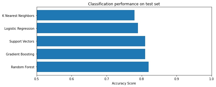
An 82% accuracy and F1 score, not bad.
              precision    recall  f1-score   support

        open       0.54      0.38      0.44        56
       bongo       0.89      0.32      0.47        25
      shaker       0.70      0.42      0.52        38
         rim       0.72      0.60      0.66       108
        snap       0.79      0.63      0.70        30
        clap       0.79      0.74      0.76       215
         hat       0.77      0.86      0.81       395
       snare       0.79      0.86      0.83       484
         tom       0.87      0.84      0.86       327
       crash       0.93      0.81      0.87        68
        ride       0.95      0.80      0.87        71
        kick       0.90      0.94      0.92       509

    accuracy                           0.82      2326
   macro avg       0.80      0.68      0.73      2326
weighted avg       0.82      0.82      0.82      2326
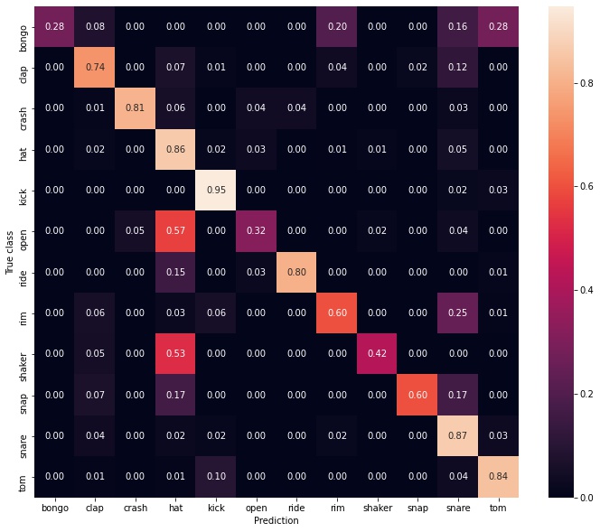
As you can see, performance on the test set really depends on the drum class. Open hi-hats and bongos are difficult, while kicks are easily classified (not surprising, because their lower frequency presence is unique). For a better understanding of the model’s misclassifications, lets look at a confusion matrix. The following is normalized by row, so for example 8% of the time bongos are confused as claps.
One reason I like using Random Forest models is their ability to give insight into which features were most useful for differentiating between classes. In this case, 72 features is way too many to comprehend in one chart, but we can group most of them into feature sets:
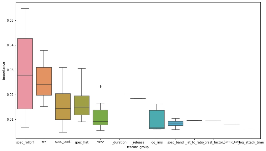
Spectral rolloff features are very important because they help differentiate sounds at the extremes of the frequency spectrum. The next most important are the remaining spectral features, Zero Crossing Rate, and a small number of outlier MFCC features. The MFCC distribution makes sense because they represent coefficients of a series of terms that get smaller and smaller; while the first few MFCCs explain a lot of the data, as you include more they represent coefficients of smaller less explanatory terms.
Method 2: Convolutional Neural Networks
A major trend of ML in the past decade has been the abandonment of higher-level hand-crafted features in favor of deep neural networks that do their own feature engineering over lower-level signals. A particularly powerful family of these is the Convolutional Neural Network (CNN), which rose to prominence in the Computer Vision field but quickly found a home in other domains too, like language and music.
How do they work? A CNN uses a bunch of smaller filters to find patterns in spatial or temporal data. As an example, if you were working with images, a single filter might represent something like a horizontal line sitting in a 3x3 pixel window. A “convolution” is an operation that essentially moves a filter window across an image, scanning for matches and returning a score representing how close each part of the image is to the filter.
An example convolution. A 3x3 filter is scanned over the blue array, with each green square representing an activation score (Source)
In practice, the situation is more complicated:
- you will use dozens or even hundreds of filters that each specialize in a different pattern
- the filter patterns will be determined automatically by a backpropagation learning procedure
- after the convolution operation you typically add additional layers, such as: batch normalizations, nonlinearities to give the neural net more expressive power, and pooling layers such a max pool which essentially turns “where in the input is this pattern the strongest?” into “does this pattern appear?”
- often people stack multiple convolutional + pooling layers on top of each other. In this case, you can think of the higher-level ones as looking for patterns of patterns.
- for classification problems, we add standard fully-connected layers atop the convolutional layers, and finally a softmax function that outputs a probability for each drum class.
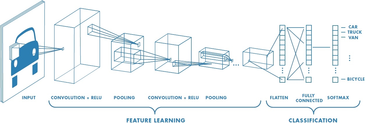
Example of a CNN architecture (Source)
All examples above operate on two dimensional inputs, but the same concept could apply in one dimension to audio data – instead of scanning up and down, the filters are also one dimensional, and are scanned beginning to end. That said, I decided to use two dimensional Mel Spectrograms following the lead of research papers I came across. These are similar to the spectrograms we looked at above, but they use an alternate frequency axis that more closely reflects the way humans hear sounds.
After some testing I settled on an architecture with two convolutional layers and two linear layers. Here’s what my PyTorch implementation looks like:
class ConvNet(nn.Module):
    def __init__(self):
        super(ConvNet, self).__init__()
        self.conv1 = nn.Conv2d(1, 256, kernel_size=(12, 4), stride=2)
        self.conv1_batch = nn.BatchNorm2d(256)
        self.conv2 = nn.Conv2d(256, 256, kernel_size=(4, 4), stride=(1, 2))
        self.conv2_batch = nn.BatchNorm2d(256)
        self.fc1 = nn.Linear(512, 128)
        self.fc2 = nn.Linear(128, len(DRUM_TYPES))

    # x is a Tensor object of size 1x128x259 containing normalized mel spectrogram data
    def forward(self, tensor, softmax=True):
      # First convolution
      tensor = F.leaky_relu(
          F.max_pool2d(
              self.conv1_batch(self.conv1(tensor)),
              stride=(4, 4)
          )
      )
      # Second convolution
      tensor = F.leaky_relu(
          F.max_pool2d(
              self.conv2_batch(self.conv2(tensor)),
              stride=(4, 8)
          )
      )

      # Now two fully connected layers, and a softmax
      assert np.prod(tensor.shape[1:]) == 512
      tensor = tensor.view(-1, 512)
      tensor = F.leaky_relu(self.fc1(tensor))
      tensor = F.dropout(tensor, training=self.training)
      tensor = self.fc2(tensor)

      return F.log_softmax(tensor, dim=-1) if softmax else tensor
One downside of applying deep neural networks to low-level data is the extra processing required. It helps that due the parallel nature of convolutions we can use a GPU instead of a CPU, which makes this feasible. Still, it took me 3-4 hours to train on an RTX 2080 Ti.
To run this yourself:
python drum_sound_classifier/models/train_cnn.py

train_cnn.py [-h] [--batch_size BATCH_SIZE]
                    [--val_batch_size VAL_BATCH_SIZE]
                    [--max_epochs MAX_EPOCHS]
                    [--early_stopping EARLY_STOPPING] [--lr LR]
                    [--momentum MOMENTUM] [--max_per_class MAX_PER_CLASS]
                    [--log_interval LOG_INTERVAL]
                    [--continue_name CONTINUE_NAME] [--eval]
From these training curves, you can see my model generally got better after each training epoch:
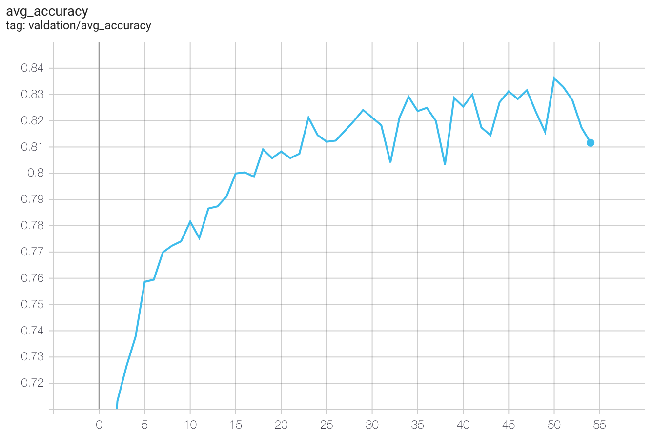
Validation accuracy during training. The x-axis is the number of epochs, y-axis is accuracy
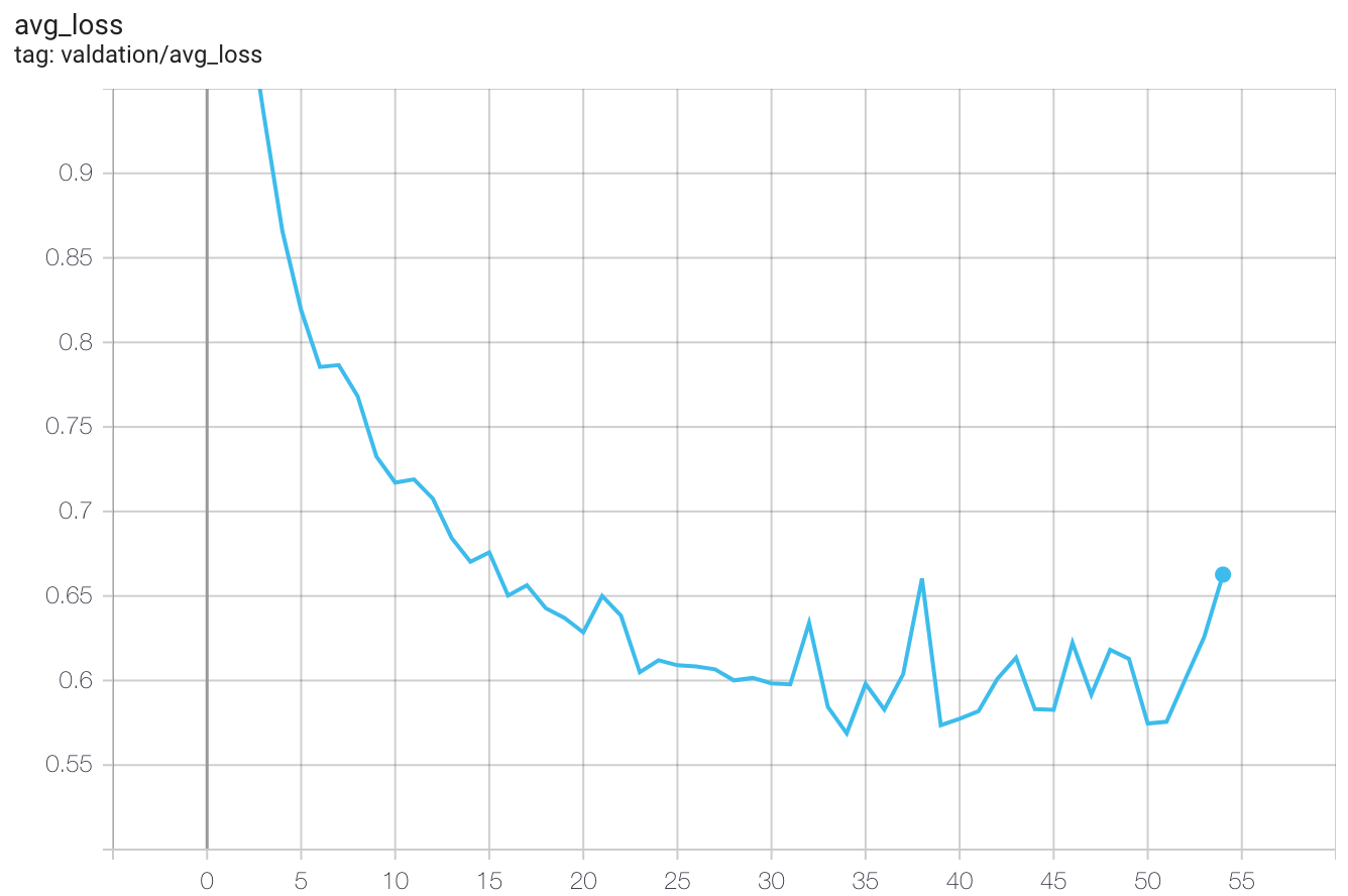
Negative log likelihood loss on the validation set
There is a spike in accuracy of 83.62% on the 50th epoch, a slight improvement over method 1. Let’s keep going!
Method 3: CNN features + SVM
Using method 1 I showed that a handful of hand-crafted features and a Random Forest classifier does pretty well. With method 2, I showed that CNNs can discover their own hierarchical feature representations, which make them even more effective.
The CNN architecture offers a few points of interception where instead of running inputs through the entire pipeline, one can stop to measure their values coming out of a particular layer. In my own architecture, the second convolutional layer results in 512 values, which gets fed into a linear layer that outputs 128 values, which then gets fed through another linear layer down to 12 (the number of drum types). At each of these points, I can intercept the values and use them as a general-purpose embedding representation of a drum input.
What would happen if I fed the 512 or 128 sized embeddings into a Random Forest or other standard ML classifier? On one hand, the pure CNN solution might have an advantage in that the model we’re putting in front of the embeddings (the final linear layer followed by softmax), is the exact same model setup that was used during the training procedure to optimize the embeddings themselves. It would be like if some engineers built a specialized engine for a particular high-end car – what are the chances some other car runs it better?
But on the other hand, the Random Forest frontend has already shown promise with less complex data, and it has the benefit of being an ensemble method which should make it more robust.
To get size-128 embeddings from the CNN all I had to do was add a method similar to forward(), but that stops after the first fully-connected layer.
def embed(self, tensor):
    tensor = F.leaky_relu(
        F.max_pool2d(
            self.conv1_batch(self.conv1(tensor)),
            (4, 4)
        )
    )
    tensor = F.leaky_relu(
        F.max_pool2d(
            self.conv2_batch(self.conv2(tensor)),
            (4, 8)
        )
    )
    assert np.prod(tensor.shape[1:]) == 512
    tensor = tensor.view(-1, 512)
    return F.leaky_relu(self.fc1(tensor)).detach().numpy()[0]
And now, I can feed these into scikit-learn like any other dataset.
To do this yourself, assuming you ran all the above commands:
python drum_sound_classifier/models/train_sklearn.py --inputs cnn_embeddings --model random_forest --max_per_class 2000
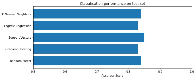
Interestingly, with a Support Vector Machine classifier the accuracy is now 85% – an improvement over the pure CNN strategy!
Inspecting model misses
Like with any classification or regression problem, it’s wise to take a closer look at instances the model struggles with.
Filenames said snare, but my model said otherwise:
Filenames said hat, but my model said otherwise:
Filenames said tom, but my model said otherwise:
There are a few different things happening here. Remember how I decided to trust the filenames of drum kits as the ground truth labels? Well, some of them are obviously wrong (like any of the toms above). Not only can this degrade my model’s performance, but it obfuscates it so the true accuracy is not known. Dataset cleaning doesn’t make for great blog content so I will spare you, but at this point before exploring any additional model architectures, it would be worth manually annotating such discrepancies.
Some of the examples above do reveal straight-up mistakes by the model, but others are less clear cut and reasonable people could disagree about the true class (the third snare above – snare or clap?). Ultimately, the boundaries between drum types are blurry so 100% accuracy is not a reasonable goal.
Conclusion
It’s possible to turn a disorganized pile of drum sounds into a dataset well-suited for ML. And, there are a few standard approaches for training a classifier of drum types that achieve good accuracy.
One takeaway that can be applied to other domains is that if you have hand-crafted features readily available that you think will capture the contours of your problem, throwing standard classification tools at it can be the best bang for your buck. You typically require fewer data, it’s easier to implement, and you can avoid high training costs.
Another takeaway is that sometimes CNNs (and deep neural networks in general) are best viewed as feature extractors, not merely as end-to-end models. This is particularly true when the neural net is trained for the problem of interest, or a similar problem. I also tried putting a Random Forest in front of features derived from a convolutional autoencoder, but didn’t see the same gains.
So what’s next? How can we do better? One way might be to use a WaveNet, a special type of CNN that applies dilated convolutions to a raw audio signal. WaveNets have proven themselves very effective as generative models for applications like speech synthesis or even drum synthesis. But they can also be applied in a classification setting. This may be the subject of a future blog post.
Data augmentation would make for another quick win. The idea is to systematically modify training examples to increase the diversity of data seen by the model, and thus increase its robustness. In the audio ML field, one way to do this is random pitch shifts or time stretches.
Here are some uses I’ve gotten out of my drum classification model:
- corrected mislabeled sounds by writing new filenames
- projected drum embeddings down to two dimensions and plotted them, for an interesting new method of browsing through sounds
- outlier detection to come up with “safe” random drum racks
References
- O. Gillet. Transcription des signaux percussifs. Application à l’analyse de scènes musicales audiovisuelles. PhD thesis, 2007.
- P. Herrera, A. Yeterian, R. Yeterian and F. Gouyon. Automatic classification of drum sounds: a comparison of feature selection methods and classification techniques” Perfecto Herrera, Alexandre Yeterian, Fabien Gouyon. 2002.
- E. Pampalk, P. Herrera, M. Goto. Computational Models of Similarity for Drum Samples. 2008
- X. Zhang, Y. Gao, Y. Yu, W. Li. Music Artist Classification with WaveNet Classifier for Raw Waveform Audio Data. 2020.
- Neural Drum Machine - An interactive system for real time synthesis of drum sounds
- https://musicinformationretrieval.com/