<?xml version="1.0" encoding="utf-8"?><feed xmlns="http://www.w3.org/2005/Atom" ><generator uri="https://jekyllrb.com/" version="4.3.4">Jekyll</generator><link href="https://soundsandwords.io//feed.xml" rel="self" type="application/atom+xml" /><link href="https://soundsandwords.io//" rel="alternate" type="text/html" /><updated>2025-11-03T21:25:30+00:00</updated><id>https://soundsandwords.io//feed.xml</id><title type="html">Sounds and Words</title><subtitle>Applying data science and ML to audio and language</subtitle><author><name>Evan Radkoff</name></author><entry><title type="html">What did you agree to? Readable privacy policies with help from ML</title><link href="https://soundsandwords.io//privacy-policies/" rel="alternate" type="text/html" title="What did you agree to? Readable privacy policies with help from ML" /><published>2025-05-18T00:00:00+00:00</published><updated>2025-05-18T00:00:00+00:00</updated><id>https://soundsandwords.io//privacy-policies</id><content type="html" xml:base="https://soundsandwords.io//privacy-policies/"><![CDATA[<p>You read the Terms &amp; Conditions, right? You didn’t just click the checkbox? And the Privacy Policy, you understood everything in there?</p>

<p>Neither did I. These kinds of documents are supposed to inform us of how our data is handled and the rights we have when using a website or app. Unfortunately, they’re usually either an unintelligible soup of legalese, or so long that they’d take a full afternoon to read. Companies have little incentive to provide summaries – they’re usually just filling a legal requirement.</p>

<p><a href="https://tosdr.org/">Terms of Service; Didn’t Read</a> (ToS;DR) has been trying to fix this. For each digital service they provide a collection of statements in yes/no format – for example, <a href="https://edit.tosdr.org/cases/129">“This service tracks you on other websites”</a> – that together offer a decent summary of the service’s policies. They even aggregate these statements into overall grades (Wikipedia <a href="https://tosdr.org/en/service/265">gets a “B”</a>), and offer <a href="https://tosdr.org/en/sites/download">browser extensions</a> so you can see grades as you browse the Web.</p>

<p><img src="/images/privacy/wikipedia_points.png" alt="Some of the summary statements about Wikipedia's terms of service available on tosdr.org" style="width: 400px; text-align: center;" /></p>

<p>Historically ToS;DR has relied solely on volunteers to do the tedious work of reading and annotating privacy documents. This is a heavy bottleneck on coverage. To date it has around 10,000 websites and apps catalogued, only ~8,600 of which are graded. It’s a great start, but it obviously falls short given how many websites and apps are out there handling your data.</p>

<p><span class="caption">
<img src="/images/privacy/grades.png" alt="Number of services on tosdr.org, by privacy grade. N/A means there are not enough known summary points to even assign a grade." style="text-align: center;" /><br />
The vast majority of websites on ToS;DR have yet to be graded. Data from December 2024.
</span></p>

<h2 id="automation">Automation</h2>

<p>To help, I teamed up with ToS;DR to scale their efforts of annotating and scoring privacy agreements with help from AI, a solution we call Docbot.</p>

<p>Specifically, I’ve used the human annotations collected over the years to train classification models that can estimate the strength of evidence for particular statements in privacy documents. If the models find evidence that scores above a certain threshold, the relevant excerpts are submitted to human curators. Once approved, the statement summaries are used automatically when calculating grades.</p>

<p><span class="caption">
<img src="/images/privacy/curator_queue.png" alt="A preview of the queue shown to human curators who can approve or reject Docbot submissions." style="width: 700px; text-align: center;" /><br />
The output of Docbot – a queue of observations about privacy documents for human curators to later approve or reject. ‘Rating’ refers to whether the observation is a positive or negative thing for privacy, while ‘Score’ refers to the strength of evidence.
</span></p>

<p>In the remainder of this post I’ll share my experience developing the solution and ultimately putting it to use within ToS;DR.</p>

<h1 id="the-methodology">The Methodology</h1>

<p>As mentioned above, ToS;DR has come up with a taxonomy of privacy-related statements that you might want to know about a digital service. We call these <em>Cases</em>, and here are some examples:</p>
<ul>
  <li>Your personal data is not sold</li>
  <li>You must provide your legal name, pseudonyms are not allowed</li>
  <li>Tracking cookies refused will not limit your ability to use the service</li>
  <li>Your data is processed and stored in a country that is less friendly to user privacy protection</li>
  <li>The terms for this service are easy to read</li>
  <li>… and <a href="https://edit.tosdr.org/cases">over 100 more</a></li>
</ul>

<p>For each Case I trained a binary classification model that takes as input one or more sentences, and outputs a 0.0-1.0 score where 1.0 means there is extremely strong evidence that the Case statement is true. Like many other text classification problems, this was a good fit for fine-tuning.</p>

<p>Key to this approach was that not only did ToS;DR have data on which Cases are present in which documents, but specifically which excerpts provide the evidence. These can fit inside the context windows of transformer models during training, and most importantly, our solution can try different excerpts to find any that are high-scoring enough for submission to ToS;DR curators. Ideally, these AI submissions will look indistinguishable from those submitted by humans.</p>

<p>Sentence classification is a common problem in NLP, and this is almost that. There were two differences here that I had to figure out: 1) we wanted to apply the models to <em>full</em>
terms of service documents and privacy policies, often with many thousands of words. We only wanted to extract the most convincing excerpt, even if multiple sentences in the document were relevant. And 2) sometimes policies are communicated in short paragraphs instead of single sentences, and we ideally wanted to preserve these spans of text as logical units, instead of only working at the single sentence level. Put another way: the problem actually sits somewhere between sentence classification and document classification.</p>

<p>My solution for inference (using the models) was:</p>
<ul>
  <li>Split the document into sentences</li>
  <li>Apply the model to each sentence individually</li>
  <li>Take the highest scoring sentence, and see if appending additional neighboring sentences makes the score go up (until some limit, e.g. 5). If so, keep them.</li>
  <li>See if prepending prior neighboring sentences makes the score go up even more. If so, keep them.</li>
  <li>Use the final sentence span and score as the result for the document.</li>
</ul>

<h2 id="forming-datasets">Forming Datasets</h2>

<p>Much of the work for supervised classification approaches like this lies in designing effective training and evaluation datasets.</p>

<p>At the very least I needed a dataset of sentence spans to train each binary classifier, with positive and negative examples. These datasets could also be useful for evaluating models, but they didn’t seem fully adequate. Since our models were ultimately being applied to entire policy documents, I formed a companion dataset of full documents to evaluate against. For one, the accuracy metrics would be much more intuitive compared to the sentence span dataset with different class ratios. But also, it would evaluate my models in the same context in which they will be used in the real world, with the “highest score” inference procedure described above.</p>

<h3 id="sentence-span-dataset">Sentence Span Dataset</h3>
<p>Positive examples here were easy – each Case had a collection of verified quotes submitted by ToS;DR volunteers over the years, sometimes in the hundreds. I decided to only tackle Cases for which we had at least 40 positive examples, leading to 123 Case models in total. The remaining could some day be covered using other text classification methods like <a href="https://arxiv.org/abs/2209.11055">SetFit</a> or few-shot prompting LLMs.</p>

<p><img src="/images/privacy/pos_instances.png" alt="Distribution of the number of positive training examples per model. Most have under 150, and nearly all have under 250." style="text-align: center;" /></p>

<h4 id="negative-examples">Negative examples</h4>
<p>These were trickier. Obviously with such long documents, searching for proof of individual Case statements is like finding a needle in a haystack, and so there is plenty of hay – completely irrelevant sentence spans. One problem to be aware of is extreme class imbalance; sampling uniformly from entire documents would probably not end well.</p>

<p>The other big problem is that we don’t just want models to lazily learn to recognize the topic of a case. For example, we don’t want a model learning the case “Tracking cookies refused will not limit your ability to use the service” to just score highly any time it sees a statement about cookies. The solution here is to expose the model to plenty of “hard negatives”, which contain similar terms and force the model to more carefully discriminate.</p>

<p>For each case I put together a set of negative examples containing:</p>
<ul>
  <li>Human submissions that were later rejected</li>
  <li>Sentence spans that surround positive examples. This approach is prone to accidental true negatives, but I believe it should help to sharpen the discriminative power of models.</li>
  <li>The ToS;DR taxonomy actually groups cases into <a href="https://edit.tosdr.org/topics">topics</a>, so I included approved submissions from other related cases</li>
  <li>Other random sentence spans from documents containing positive examples</li>
  <li>Random sentence spans from comprehensively reviewed documents that do not contain positive examples</li>
</ul>

<p>Another helpful source of negative examples could come from manually constructing logical negations of positive examples. Assertions that data practices are <em>not</em> carried out are rare, but they exist. Using negations could lead to more robust models that can handle these correctly – instead of just learning phrases, they would have to learn to analyze the statement’s modality. I didn’t include these in our first model versions, but a similar project called MAPS[1] took this approach.</p>

<p>Another future direction is hard negative mining with vector similarity search, which would help surface examples right on the edge of what we’re trying to learn.</p>

<h4 id="sentence-length-bias">Sentence length bias</h4>

<p>When constructing training examples, it’s important not to introduce any unintended biases. The models should learn to discriminate between positive and negative examples by way of learning the underlying task at hand, rather than learning irrelevant characteristics of the constructed examples that you introduced.</p>

<p>For example, here the human submitted quotations (positive training instances) could be any number of sentences. If our constructed negative instances were only one sentence, a model could theoretically learn the rule “If I’m shown multiple sentences, it’s positive.”</p>

<p><img src="/images/privacy/num_sents.png" alt="Distributions of the number of sentences found in human submitted quotes that provide evidence for a few random cases. Some typically have one sentence, others commonly have 3, 4, even 5 sentences." style="text-align: center;" /></p>

<p>My solution here was to model each case’s typical number of sentences for submitted evidence as a multinomial probability distribution, and sample from it while constructing negative instances.</p>

<p>Another potential source of bias is that submissions don’t necessary have to begin and end at sentence boundaries – people can highlight partial sentences, even short phrases. Rather than try to replicate typical start and end times for each case, I decided to just expand positive instances to begin and end at their surrounding sentence boundaries. This restricts the resulting models to also only yield full sentence predictions, but that’s fine, and it avoids any related bias issue.</p>

<h3 id="document-dataset">Document Dataset</h3>

<p>The dataset of full documents (privacy policies, terms and conditions, cookie policies, etc.) was more straight-forward. Positive instances were those which had an approved submission of evidence from ToS;DR volunteers. Negative instances included documents that were comprehensively reviewed by volunteers without the case ever coming up, or rejected submissions if there were any.</p>

<p>This was utilized for evaluation only, using my custom “sentence expansion” inference procedure. It correlated with performance on the sentence span dataset used for training, but I think it’s more trustworthy for model selection because it’s closer to how we use the models downstream.</p>

<p>The only “gotcha” was to prevent data leakage by stratifying train/test splits the same way I did for the sentence span dataset: by website/service. I first split services into two groups 80-20, and then partitioned both datasets accordingly.</p>

<h1 id="training-docbot">Training Docbot</h1>

<p>I relied on the tried-and-tested fine-tuning of BERT family models using huggingface. <a href="https://huggingface.co/bert-base-uncased">bert-base-uncased</a>, <a href="https://huggingface.co/roberta-base">roberta-base</a>, and a finetune of legal documents <a href="https://huggingface.co/nlpaueb/legal-bert-base-uncased">legal-bert-base-uncased</a> all performed about the same. <a href="https://huggingface.co/blog/modernbert">ModernBERT</a> looks great, but wasn’t yet released at the time of training. Rather than fine-tuning the full base models I decided to train more parameter efficient LoRA adapters [2], via the huggingface <a href="https://github.com/huggingface/peft">peft</a> library.</p>

<p>Interestingly the vast majority of time spent during training was actually the evaluation loop, when full documents were analyzed. This could surely be sped up by not re-running obviously unrelated sentences, but that’s an optimization for another day. This means using LoRAs didn’t actually have much of an effect on training speed, but they were still nice for disk space efficiency (each of the 123 models is just a 2.8MB adapter file), and there was virtually no reduction in accuracy compared to a full fine-tune.</p>

<p>As is typical when fine-tuning LLMs, accuracy can differ a decent amount depending on the random seed. This means it was beneficial to attempt training each Case multiple times, taking the highest test set accuracy observed across all attempts.</p>

<p>Training was carried out on <a href="https://cloud.vast.ai/">vast.ai</a> instances, using <a href="https://wandb.ai">Weights &amp; Biases</a> to track experiments and visualize metrics.</p>

<p><span class="caption">
<img src="/images/privacy/training_curves.png" alt="Training curves showing multiple restarts of fine-tuning one case model in particular -- &quot;You maintain ownership of your content&quot;. The x-axis shows the number of training steps, and the y-axis shows F1 score on the test set of the full document dataset. Some attempts did better than others but they are all within .05-.1 of each other." style="width: 650px; text-align: center;" /><br />
Training curves for multiple restarts of one case model in particular – “You maintain ownership of your content”. The y axis shows F1 score on the test set fold of the full document dataset.
</span></p>

<h3 id="what-about-just-prompting-llms">What about just prompting LLMs?</h3>
<p>Few-shot prompting is another way to perform text classification. Sometimes it’s the right tool for the job, especially when training data is hard to come by and you want a quick solution. For this problem I opted for fine-tuning because of it’s potential for higher accuracy at low cost, and because it provides interpretable and reliable confidence scores with each prediction.</p>

<p>LLMs could still be useful to help bootstrap Cases with very few training examples, and to audit training datasets for true negatives.</p>

<h2 id="model-and-threshold-selection">Model and threshold selection</h2>

<p>I used early stopping to halt training, and selected the model checkpoint that maximized F1 on the full document dataset across all restarts.</p>

<p>One benefit of using regression models or neural networks for classification is that we can choose prediction thresholds at our preferred place on the precision-recall curve. Since we planned to send AI submissions to human curators before use in privacy grades, a lower threshold was preferable. This would mean more false positives crowding the approval queue (lower precision), but would ensure better coverage finding matches (higher recall).</p>

<p>I found that a single static post-softmax probability threshold would not work across Case models, as they were not very consistent in their relative implied confidence. And with 123 models in total, it was best to automate threshold selection by maximizing an objective criteria. <a href="https://en.wikipedia.org/wiki/F-score">F-score</a> is a great choice because it incorporates both precision and recall and allows us to specify a tradeoff preference using the beta parameter. In my case I used a beta of 1.5 to prefer recall. The charts below show precision-recall curves and the corresponding f-scores as we vary the classification decision thresholds from 0.0 to 1.0.</p>

<p><span class="caption">
<img src="/images/privacy/thresholds.png" alt="Precision-recall curves of five different Case models, along side a chart showing their corresponding f-scores as a function of 0.0-1.0 classification decision thresholds." style="width: 750px; text-align: center;" /><br />
On the left, precision-recall curves of five different case models. On the right, available f-scores for the same models, as a function of the decision threshold that could be used for classification. A black X marks the optimal point.
</span></p>

<h2 id="results">Results</h2>

<p>Model accuracy varied quite a bit by Case.</p>

<p><span class="caption">
<img src="/images/privacy/pr.png" alt="A scatterplot showing precision and recall for all 123 case models. Recall is typically above .7, while precision is more varied typically ranging between .3 and .75" style="width: 500px; text-align: center;" /><br />
Precision and recall for all 123 Case binary classification models.
</span></p>

<p>Sorting by f-score shows us the best and worst performing models:</p>

<table>
  <thead>
    <tr>
      <th style="text-align: right">F-score</th>
      <th style="text-align: left">Case</th>
    </tr>
  </thead>
  <tbody>
    <tr>
      <td style="text-align: right">0.942</td>
      <td style="text-align: left">The service is provided ‘as is’ and to be used at your sole risk</td>
    </tr>
    <tr>
      <td style="text-align: right">0.929</td>
      <td style="text-align: left">Do Not Track (DNT) headers are ignored and you are tracked anyway even if you set this header</td>
    </tr>
    <tr>
      <td style="text-align: right">0.923</td>
      <td style="text-align: left">You are tracked via web beacons, tracking pixels, browser fingerprinting, and/or device fingerprinting</td>
    </tr>
    <tr>
      <td style="text-align: right">0.919</td>
      <td style="text-align: left">You waive your right to a class action</td>
    </tr>
    <tr>
      <td style="text-align: right">0.884</td>
      <td style="text-align: left">You have a reduced time period to take legal action against the service</td>
    </tr>
    <tr>
      <td style="text-align: right">…</td>
      <td style="text-align: left">…</td>
    </tr>
    <tr>
      <td style="text-align: right">0.455</td>
      <td style="text-align: left">Private messages can be read</td>
    </tr>
    <tr>
      <td style="text-align: right">0.443</td>
      <td style="text-align: left">You cannot distribute or disclose your account to third parties</td>
    </tr>
    <tr>
      <td style="text-align: right">0.430</td>
      <td style="text-align: left">The terms for this service are easy to read</td>
    </tr>
    <tr>
      <td style="text-align: right">0.363</td>
      <td style="text-align: left">Logs are kept for an undefined period of time</td>
    </tr>
    <tr>
      <td style="text-align: right">0.328</td>
      <td style="text-align: left">A free help desk is provided</td>
    </tr>
  </tbody>
</table>

<p>Prediction accuracy was higher for more strictly defined Cases that often use consistent language across privacy documents. Accuracy was lower for Cases with lots of edge cases, or ones with lower quality training sets.</p>

<p>When it comes to the quoted evidence submitted for approval, generally the Docbot submissions looked just like those from humans. They did tend to be a little longer on average, in part because they had to adhere to sentence boundaries, but also because too many sentences were appended during the inference procedure. The chart below shows differences in distributions of the number of sentences for a few random Cases, and you can see some are worse than others. This can be refined in future versions.</p>

<p><img src="/images/privacy/num_sents_docbot.png" alt="Distributions of the number of sentences found in human submitted vs Docbot submitted quotes that provide evidence for a few random Cases. The distributions are generally similar, but Docbot submissions are sometimes longer." style="text-align: center;" /></p>

<h1 id="the-rollout">The Rollout</h1>

<p>There was no need to have our models hosted as an API, since we just need to apply them once for each privacy document as a batch job. New services and documents are added to ToS;DR regularly, and so we can re-run the inference jobs daily or weekly.</p>

<p>To keep track of which documents have been already been analyzed by Docbot, we added a new database table that stores the results of inference: document ID, Case ID, Docbot version, the start and end character positions of the highest-scoring sentence span, and the probability score. This allows for audits and keeps us from running the same model on the same document twice. In the future we’ll likely also use a job queue to facilitate inference parallelization.</p>

<p>I also decided to have the inference job re-consider documents for which the human curators rejected a previous submission. If Docbot (or a human) thinks it found evidence for a Case but was wrong, that doesn’t mean evidence doesn’t exist elsewhere in the document. Previously rejected sentence spans act as “off limits” areas during inference.</p>

<p>After setting up APIs for Docbot to interact with the ToS;DR backend, we made a new frontend for the Docbot submission queue. Once again here’s what that looks like:</p>

<p><span class="caption">
<img src="/images/privacy/curator_queue.png" alt="A preview of the queue shown to human curators who can approve or reject Docbot submissions." style="width: 700px; text-align: center;" /><br />
A preview of the queue shown to human curators who can approve or reject Docbot submissions.
</span></p>

<p>Submissions are sorted by descending confidence score so that the most likely approvals are at the top. Curators can also filter by Case, if they just want to churn through the results of a single model.</p>

<h2 id="the-impact">The Impact</h2>
<p>ToS;DR only assigns privacy grades to a service when it has enough knowledge about its policies, meaning it has enough approved evidence submissions. Thanks to Docbot, the bottleneck on grade coverage has now shifted from volunteers initially reading through and annotating documents, to volunteer curators that double-check submissions as a final sign-off.</p>

<p><span class="caption">
<img src="/images/privacy/number_of_points.png" alt="The number of evidence submissions over time from both humans and Docbot, featuring a huge increase from 38,000 to 120,000 from the first runs of Docbot." style="width: 450px; text-align: center;" /><br />
The number of submissions of evidence for Cases from either humans or Docbot over time. The two big jumps to the right are from the first runs of Docbot. By the time remaining Cases are run, we expect there to be over 300,000.
</span></p>

<p>In the coming months we’ll explore ideas for easing that bottleneck, such as:</p>
<ul>
  <li>A Tinder-style swiping interface for approving or rejecting Docbot submissions more quickly on the go. We do have to be careful to make sure curators still apply enough scrutiny, for example by having redundent approvals and measuring <a href="https://en.wikipedia.org/wiki/Inter-rater_reliability">inter-rater reliability</a>.</li>
  <li>Rather than working through giant queues of submissions, encouraging curators to go service-by-service to increase grade coverage more quickly, starting with the most popular ungraded services.</li>
</ul>

<p>Beyond optimizing the approval process workflow, we are also exploring options for how to incorporate Docbot more directly:</p>
<ul>
  <li>Publishing fully automated grades for services, when we don’t yet have enough human-approved submissions</li>
  <li>For very high confidence predictions (say, a score &gt;.99) we could auto-approve</li>
</ul>

<p>They key challenges with both of these approaches are to 1) choose the right score thresholds to balance false-positives with coverage, 2) have an understanding of model biases, and their effect on end grades, and 3) adequately communicating everything to our users and API consumers. People have grown to trust ToS;DR, and ultimately any incorporation of AI has to be done carefully to maintain that trust.</p>

<h1 id="conclusion">Conclusion</h1>

<p>This was a really fun side project. I got to work with a unique dataset, help solve a real world pain point, and contribute to free and open source software. Part way through this experience, I was invited to join the core dev team at ToS;DR.</p>

<h2 id="future-directions">Future directions</h2>
<p>I previously mentioned how we’d like to apply Docbot more directly by assigning tentative grades using fully automated analyses. And, we’d like to build better interfaces for double checking Docbot submissions. Beyond that, there is still so much to do!</p>

<ul>
  <li>More efficient inference, by doing a first pass that excludes paragraphs with no remote relevance to the Case topic.</li>
  <li>Use Docbot to audit for mistakenly approved points already in ToS;DR</li>
  <li>Automated retraining of models, CI/CD</li>
  <li>Expand coverage to non-English languages</li>
  <li>Expand coverage to Cases with very few training examples</li>
  <li>Release datasets for NLP and legal researchers, open source the LoRA adapters</li>
  <li>Put out a tool to help service owners craft their privacy docs to be more privacy friendly, by getting feedback in real time</li>
  <li>Beyond binary statements, extract targeted information from privacy docs, like a list of what data are collected, and how long the service keeps it</li>
</ul>

<h3 id="other-things-that-would-help-with-digital-privacy">Other things that would help with digital privacy</h3>
<ul>
  <li>Crawling the web to automatically add services and privacy docs</li>
  <li>Regulation for companies to provide easier to understand summaries, as <a href="https://ico.org.uk/for-organisations/guide-to-data-protection/guide-to-the-general-data-protection-regulation-gdpr/principles/lawfulness-fairness-and-transparency">GDPR does</a>, and protocols for machine-readable policies, as <a href="https://standards.ieee.org/ieee/7012/7192/">IEEE proposes</a></li>
  <li>Tracking data leaks and privacy scandals</li>
</ul>

<p>If you found this project interesting you can help us by contributing analyses on <a href="https://edit.tosdr.org/">edit.tosdr.org</a>, <a href="https://tosdr.org/en/contact">getting in touch</a> to contribute to development, or even <a href="https://tosdr.org/donate">donating</a>.</p>

<p><br /></p>

<div class="ad">
  <div class="ad-column-left">
    <p>
      <p>Have some data and a problem to solve?</p>
      <p>I'm available for consulting and contract work.</p>
      <p><a href="/consulting">Learn more</a></p>
    </p>
  </div>
  <div class="ad-column-right">
    <div class="icon-container">
      <a href="mailto:evan@soundsandwords.io">
        <i class="svg-icon-large email-large"></i>
      </a>
    </div>
  </div>
</div>

<h4 id="references">References</h4>

<ul class="bib">
  <li>[1] S. Zimmeck. MAPS: Scaling Privacy Compliance Analysis to
a Million Apps, 2019.</li>
  <li>[2] E. Hu. LoRA: Low-Rank Adaptation of Large Language Models, 2021.</li>
</ul>]]></content><author><name>Evan Radkoff</name></author><category term="Text Classification" /><category term="Machine Learning" /><category term="Legal Documents" /><category term="Summarization" /><summary type="html"><![CDATA[Training text classifiers on privacy policies and terms and conditions to help reclaim privacy.]]></summary><media:thumbnail xmlns:media="http://search.yahoo.com/mrss/" url="https://soundsandwords.io//images/consulting/tosdr.png" /><media:content medium="image" url="https://soundsandwords.io//images/consulting/tosdr.png" xmlns:media="http://search.yahoo.com/mrss/" /></entry><entry><title type="html">The Unreasonable Power of Vectors</title><link href="https://soundsandwords.io//the-unreasonable-power-of-vectors/" rel="alternate" type="text/html" title="The Unreasonable Power of Vectors" /><published>2024-10-26T00:00:00+00:00</published><updated>2024-10-26T00:00:00+00:00</updated><id>https://soundsandwords.io//the-unreasonable-power-of-vectors</id><content type="html" xml:base="https://soundsandwords.io//the-unreasonable-power-of-vectors/"><![CDATA[<p>Let’s say you have a dataset of Things. Things could be people, cities, countries, dinosaurs, episodes of The Simpsons, whatever really. You’d like to better understand the dataset as quickly as you can, use it to improve your understanding of Things, and maybe even build software features on top of it. Basically, you want the dataset “at your fingertips”.</p>

<p>In this situation, a really useful intermediate goal is figuring out the best way to turn your dataset into vectors, essentially just lists of numbers, each denoting a dimension with meaning. Vectors represent a vital stepping stone in the standard data science process – done right, they immediately unlock several paradigms for understanding, and building on top of, your data.</p>

<p>There’s a science to designing the right vector space for your use case. Sometimes working directly with tabular features is fine, usually with some scaling/preprocessing. Other times you might want to employ a training paradigm like word2vec, neural networks, or <a href="https://scikit-learn.org/stable/modules/manifold.html">manifold learning</a>. Admittedly this post should really be called “The unreasonable power that comes with representing your dataset as well-formed vectors of mostly-independent normalized features”, that just didn’t sound as snazzy.</p>

<p>But this is not a blog post about how to <em>design</em> vector spaces. Rather, I’ll cover the things you can do once you’ve embedded your dataset as a bag of vectors. Whether these are as simple as 3-dimensional vectors describing demographics, or something complex like 4096-dimensional embeddings from the latest LLM, all of the methods below should be applicable.</p>

<h2 id="scatterplots">Scatterplots</h2>

<p>One of the most basic things you can do is visualize your dataset in 2D space. This is especially useful in the exploratory phase of a project to get your bearings, understand the dataset’s overall structure, and identify outliers.</p>

<p>Some datasets might have two features that work great as X and Y dimensions, however not all do. The key step that makes this a universally applicable approach is to automatically reduce your vectors’ dimensionality, all the way down to two, in a way that preserves their global structure. That is to say, the distances between vectors in the original high dimensional space should correlate with the distances in 2D. There are a ton of methods for doing this, each with their pros and cons. I recommend <a href="https://scikit-learn.org/stable/modules/generated/sklearn.manifold.TSNE.html">tSNE</a> or <a href="https://umap-learn.readthedocs.io/en/latest/">UMAP</a> as your go-tos.</p>

<p>Obviously a bunch of dots alone without context are not useful, but you can decorate them with a visualization framework. Point size (for numeric features), shape (for categorical features), and color (for either) offer three ways of highlighting features that help you navigate. You can also add hover tooltips, letting you see as many interpretable features as you’d like.</p>

<p>Throughout this post I’ll be demonstrating with a toy dataset of popular music. The interactive scatterplot below is derived from “genre embeddings”, 128-dimensional vectors that come from the last hidden layer of a genre classification neural network. On desktop, hover over a dot for track metadata (I couldn’t get clicking on mobile to work). Code <a href="https://github.com/radkoff/music_vectors_streamlit">available here</a>.</p>

<iframe src="https://music-vectors.streamlit.app/?embed=true&amp;embed_options=light_theme&amp;entity_choice=Tracks&amp;skip_data_sources=true&amp;skip_dim_reduction=true" style="height: 450px; width: 100%;" title="AN interactive scatterplot of genre embedding projections, for a sample of popular music tracks"></iframe>
<p><span class="caption">
Each dot represents a track from a random selection of popular music artists.
</span></p>

<p>Generally we see the tracks of artists end up near each other, which is a good sign. (As a side note, it’s also satisfying to see the dots representing Girl Talk right in between the cluster of hip-hop and other genres, because he makes mash-up music featuring hip-hop vocals over a backdrop of other genres)</p>

<p>For a much more impressive scatterplot, check out the <a href="https://atlas.nomic.ai/map/wikipedia">entirety of English Wikipedia</a> on Atlas. Enjoy the rabbit holes.</p>

<p>For those working in the Python ecosystem like myself, I can recommend <a href="https://streamlit.io/">streamlit</a> as a frontend platform with which to plot. Jupyter notebooks will work fine too, and there’s something to be said for code living right next to the plots it generates, but I find streamlit easier to work with for many use cases, including this blog post. Several plotting libraries are supported: Matplotlib, Altair, Plotly, Bokeh, and more.</p>

<h2 id="clustering">Clustering</h2>

<p>Once your dataset is in a vector space, you can always compute the distance between any two points. This could be Euclidean distance, cosine distance, or something else, but either way this simple ability unlocks a few go-to data science paradigms for free.</p>

<p>One is clustering – using an algorithm to find logical groupings. This can help you understand segments of your data, and can even work as a classifier for new data points. The <a href="https://scikit-learn.org/stable/modules/clustering.html">scikit-learn</a> library documentation offers a nice overview of common approaches. You’ll notice most of the APIs take a distance measure of your choosing as an input.</p>

<p>The shapes of the points below indicate membership in unsupervised clusters. This means they were not designed to delineate any existing  groupings, like genre labels; they were assigned according to the hands-off approach HDBSCAN. And yet, the groups do resemble genres and would be useful for downstream analysis (I’ll admit I’m cheating a little in this example.. the embeddings come from a model optimized to recognize genre, so they have a head start in ending up that way.)</p>

<iframe src="https://music-vectors.streamlit.app/?embed=true&amp;embed_options=light_theme&amp;entity_choice=Tracks&amp;skip_data_sources=true&amp;skip_dim_reduction=true&amp;cluster=true" style="height: 450px; width: 100%;" title="An interactive scatterplot of clustered genre embeddings, for a sample of popular music tracks"></iframe>
<p><span class="caption">
Like before each point represents a track, and the shape of the point is assigned according to the unsupervised clustering algorithm HDBSCAN.
</span></p>

<h2 id="similarity-search">Similarity Search</h2>

<p>Another thing you can do after choosing a distance metric is find the most similar entities to some query – a paradigm called kNN (<code class="language-plaintext highlighter-rouge">k</code> nearest neighbors), or similarity search. This can even power user-facing search features or recommendation engines. See the example below.</p>

<iframe src="https://music-vectors.streamlit.app/?embed=true&amp;embed_options=light_theme&amp;entity_choice=Tracks&amp;skip_data_sources=true&amp;skip_dim_reduction=true&amp;nn=true" style="height: 450px; width: 100%;" title="An interactive table of the most similar tracks to a query, including the Euclidian distances between 128-dimensional genre embeddings"></iframe>
<p><span class="caption">
The most similar tracks, according to the smallest Euclidian distance between 128-dimensional genre embeddings.<br />Click the dropdown to query a different track.
</span></p>

<h2 id="aggregating">Aggregating</h2>

<p>Hierarchies come up all the time with structured data. Documents are made up of paragraphs, which are made up of sentences, which are made up of words. Countries are made up of states. A customer’s activity is made up of individual actions they took.</p>

<p>Often you’ll find you want to navigate <em>up</em> these hierarchies, working with higher-level entities even though you have features/vectors for their components. Vectors allow for an elegant solution: just average each dimension, independently, across all components within a higher-level entity. A big advantage here is that it works with any number of components. For example, let’s say you’d like to measure the similarity between two documents, one with three paragraphs and one much longer with ten. Assuming you had an embedding vector for each paragraph, simply averaging the embeddings of document A’s paragraphs, and separately averaging those of document B’s paragraphs, would give you two vectors of equal length that you can measure the distance between.</p>

<p>Picking up on our example of music from above, we can average together the vectors of tracks within each album to get <em>album vectors</em>, seen below.</p>

<iframe src="https://music-vectors.streamlit.app/?embed=true&amp;embed_options=light_theme&amp;entity_choice=Albums&amp;skip_data_sources=true&amp;skip_dim_reduction=true" style="height: 450px; width: 100%;" title="An interactive scatterplot of album embeddings, by way of averaging track vectors"></iframe>
<p><span class="caption">
After aggregation, each dot now represents an album.
</span></p>

<h2 id="training-ml-models">Training ML models</h2>

<p>There are many “black box” ML paradigms that do well with inputs of arbitrary tabular data, and learn statistical patterns as needed for downstream tasks. If you’ve already done the work to represent your dataset as well-formed vectors, these downstream tasks can generally be prototyped very quickly. For example, a decent enough supervised classifier might be trainable with just an hour’s worth of labeling from a domain expert.</p>

<p>Another example of where this ease-of-application could come in handy is automated data imputation, or filling in missing values with substitutes. Imagine if a few dozen dimensions had missing values, and your goal was to generate reasonable guesses. Coming up with a unique process for each dimension could be a lot of work. However, if the vectors are in a good enough shape, you can automatically train a supervised regression model to predict each dimension of interest, iteratively holding them out as target labels and using the remaining dimensions as inputs.</p>

<h2 id="bridging-data-sources">Bridging data sources</h2>
<p>It’s not uncommon to construct datasets of entities from multiple data sources. For example, maybe each entity is a customer, and you’d like to combine demographic data with purchase history. You might have already finished an analysis, only to discover there is more data about these customers on the way.</p>

<p>The easiest way to combine such data sources is to simply concatenate their vectors. This is a good choice if your downstream application is a ML model, which ideally will learn patterns across each source.</p>

<p>In theory, all of the other tools I’ve described can also work after concatenation. One thing to be mindful of, however, is unintentionally allowing data sources with a large dimensionality to have outsized influence. Many of the methods work by computing pairwise distances between entities, and depending on your distance metric of choice, each dimension treated equally means the number of dimensions has to be considered. One way around this is instead of concatenating vectors, computing the pairwise distance matrix of each data source separately, then averaging them together so that each source has equal weight. Scikit-learn APIs generally accept distance matrices as inputs instead of raw vectors by specifying <code class="language-plaintext highlighter-rouge">metric='precomputed'</code>, as does <a href="https://umap-learn.readthedocs.io/en/latest/parameters.html#metric">umap-learn</a>. This trick also offers an opportunity to customize the influence of each source with a weight factor of your choosing.</p>

<p>The scatterplot projections below are based on the genre-describing vectors used above, in addition to high-level audio features that describe mood, provided by the <a href="https://acousticbrainz.org/">AcousticBrainz</a> API, which itself uses the <a href="https://essentia.upf.edu/algorithms_reference.html">essentia</a> library.</p>

<iframe src="https://music-vectors.streamlit.app/?embed=true&amp;embed_options=light_theme&amp;entity_choice=Tracks&amp;skip_dim_reduction=true" style="height: 550px; width: 100%;" title="An interactive scatterplot of music track vectors, from two data sources"></iframe>
<p><span class="caption">
Each dot represents a track, as represented by two different data sources – 128-dimensional genre embeddings, and 14-dimensional acoustic mood descriptors provided by AcousticBrainz/essentia.
</span></p>

<h3 id="bridging-modalities">Bridging modalities</h3>
<p>Going beyond data sources, high-level entities might be represented by multiple modes of data entirely. Text, images, videos, audio, etc. might all look very different from each other, but as long as they can be boiled down to vectors of (mostly independent) features, you can work with them together. Connecting modalities is a hot topic in modern ML (see <a href="https://arxiv.org/abs/2103.00020">CLIP</a>, used by DALL-E). But the bag-of-vectors paradigm is, I think, the easiest way to do it for limited use cases.</p>

<p>So far the example music vectors above have been made up of features extracted from raw audio. Looking for complementary data, I came across a nice <a href="https://www.kaggle.com/datasets/michaelbryantds/top-5000-albums-of-all-time-rateyourmusiccom">dataset</a> of descriptors from <a href="https://rateyourmusic.com/">rateyourmusic.com</a> – albums were labeled by human listeners according to a <a href="https://rateyourmusic.com/music_descriptor/">taxonomy</a> of atmosphere, form, lyrics, mood, style, and technique. For example, Nirvana’s <em>Nevermind</em> is labeled <code class="language-plaintext highlighter-rouge">[energetic, rebellious, angry, malevocals, apathetic, sarcastic, alienation, passionate, anxious, self-hatred]</code>. First, to get the labels into a more useful semantic vector space, I used UMAP to project the term-document matrix into 16 dimensions (I also tried Truncated SVD and PCA). These are then combined with the audio-based features from before, either at the distance matrix stage, or via concatenation in the case of PCA, while being projected down even further to two dimensions for the scatterplots below.</p>

<iframe src="https://music-vectors.streamlit.app/?embed=true&amp;embed_options=light_theme&amp;entity_choice=Albums&amp;skip_dim_reduction=true" style="height: 550px; width: 100%;" title="An interactive scatterplot of music album vectors, from three data sources"></iframe>
<p><span class="caption">
Each dot represents an album, as represented by up to three different data sources – aggregated 128-dimensional genre embeddings, aggregated 14-dimensional acoustic mood descriptors, and 16-dimensional vectors based on human labels from rateyourmusic.com.
</span></p>

<script>
window.mobileCheck = function() {
  let check = false;
  (function(a){if(/(android|bb\d+|meego).+mobile|avantgo|bada\/|blackberry|blazer|compal|elaine|fennec|hiptop|iemobile|ip(hone|od)|iris|kindle|lge |maemo|midp|mmp|mobile.+firefox|netfront|opera m(ob|in)i|palm( os)?|phone|p(ixi|re)\/|plucker|pocket|psp|series(4|6)0|symbian|treo|up\.(browser|link)|vodafone|wap|windows ce|xda|xiino/i.test(a)||/1207|6310|6590|3gso|4thp|50[1-6]i|770s|802s|a wa|abac|ac(er|oo|s\-)|ai(ko|rn)|al(av|ca|co)|amoi|an(ex|ny|yw)|aptu|ar(ch|go)|as(te|us)|attw|au(di|\-m|r |s )|avan|be(ck|ll|nq)|bi(lb|rd)|bl(ac|az)|br(e|v)w|bumb|bw\-(n|u)|c55\/|capi|ccwa|cdm\-|cell|chtm|cldc|cmd\-|co(mp|nd)|craw|da(it|ll|ng)|dbte|dc\-s|devi|dica|dmob|do(c|p)o|ds(12|\-d)|el(49|ai)|em(l2|ul)|er(ic|k0)|esl8|ez([4-7]0|os|wa|ze)|fetc|fly(\-|_)|g1 u|g560|gene|gf\-5|g\-mo|go(\.w|od)|gr(ad|un)|haie|hcit|hd\-(m|p|t)|hei\-|hi(pt|ta)|hp( i|ip)|hs\-c|ht(c(\-| |_|a|g|p|s|t)|tp)|hu(aw|tc)|i\-(20|go|ma)|i230|iac( |\-|\/)|ibro|idea|ig01|ikom|im1k|inno|ipaq|iris|ja(t|v)a|jbro|jemu|jigs|kddi|keji|kgt( |\/)|klon|kpt |kwc\-|kyo(c|k)|le(no|xi)|lg( g|\/(k|l|u)|50|54|\-[a-w])|libw|lynx|m1\-w|m3ga|m50\/|ma(te|ui|xo)|mc(01|21|ca)|m\-cr|me(rc|ri)|mi(o8|oa|ts)|mmef|mo(01|02|bi|de|do|t(\-| |o|v)|zz)|mt(50|p1|v )|mwbp|mywa|n10[0-2]|n20[2-3]|n30(0|2)|n50(0|2|5)|n7(0(0|1)|10)|ne((c|m)\-|on|tf|wf|wg|wt)|nok(6|i)|nzph|o2im|op(ti|wv)|oran|owg1|p800|pan(a|d|t)|pdxg|pg(13|\-([1-8]|c))|phil|pire|pl(ay|uc)|pn\-2|po(ck|rt|se)|prox|psio|pt\-g|qa\-a|qc(07|12|21|32|60|\-[2-7]|i\-)|qtek|r380|r600|raks|rim9|ro(ve|zo)|s55\/|sa(ge|ma|mm|ms|ny|va)|sc(01|h\-|oo|p\-)|sdk\/|se(c(\-|0|1)|47|mc|nd|ri)|sgh\-|shar|sie(\-|m)|sk\-0|sl(45|id)|sm(al|ar|b3|it|t5)|so(ft|ny)|sp(01|h\-|v\-|v )|sy(01|mb)|t2(18|50)|t6(00|10|18)|ta(gt|lk)|tcl\-|tdg\-|tel(i|m)|tim\-|t\-mo|to(pl|sh)|ts(70|m\-|m3|m5)|tx\-9|up(\.b|g1|si)|utst|v400|v750|veri|vi(rg|te)|vk(40|5[0-3]|\-v)|vm40|voda|vulc|vx(52|53|60|61|70|80|81|83|85|98)|w3c(\-| )|webc|whit|wi(g |nc|nw)|wmlb|wonu|x700|yas\-|your|zeto|zte\-/i.test(a.substr(0,4))) check = true;})(navigator.userAgent||navigator.vendor||window.opera);
  return check;
};
isMobile = window.mobileCheck();
if (isMobile) {
  document.querySelectorAll('iframe').forEach(iframe => {
      if (iframe.src) {
          iframe.src = iframe.src + "&mobile=true";
          iframe.style.height = "600px";
      }
  });
}
</script>

<h2 id="conclusion">Conclusion</h2>

<p>If you employ these paradigms enough times for enough datasets, you’ll start to <em>think</em> in vectors. “My company needs to do <code class="language-plaintext highlighter-rouge">X</code> with a bunch of <code class="language-plaintext highlighter-rouge">Y</code>s… how would I design vectors to represent <code class="language-plaintext highlighter-rouge">Y</code>s?” Or even outside of work, “I should buy a new car soon.. hmm, I wonder what car model vectors would look like?”</p>

<p>Again, the title of this post is a bit facetious. Vectors themselves are not the magic sauce, but rather a mental and practical bridge between worlds. In one world, we obsess over how to represent Things as numbers – deciding their most important features and scrutinizing data quality. In the other world, we’re able to place these numbers inside a black box, and use them to learn and build.</p>

<p><br /></p>

<div class="ad">
  <div class="ad-column-left">
    <p>
      <p>Have some data and a problem to solve?</p>
      <p>I'm available for consulting and contract work.</p>
      <p><a href="/consulting">Learn more</a></p>
    </p>
  </div>
  <div class="ad-column-right">
    <div class="icon-container">
      <a href="mailto:evan@soundsandwords.io">
        <i class="svg-icon-large email-large"></i>
      </a>
    </div>
  </div>
</div>]]></content><author><name>Evan Radkoff</name></author><category term="Data Science" /><category term="Embeddings" /><category term="Visualizations" /><summary type="html"><![CDATA[Let’s say you have a dataset of Things. Things could be people, cities, countries, dinosaurs, episodes of The Simpsons, whatever really. You’d like to better understand the dataset as quickly as you can, use it to improve your understanding of Things, and maybe even build software features on top of it. Basically, you want the dataset “at your fingertips”.]]></summary><media:thumbnail xmlns:media="http://search.yahoo.com/mrss/" url="https://soundsandwords.io//images/scatterplot.png" /><media:content medium="image" url="https://soundsandwords.io//images/scatterplot.png" xmlns:media="http://search.yahoo.com/mrss/" /></entry><entry><title type="html">Loss Functions in Audio ML</title><link href="https://soundsandwords.io//audio-loss-functions/" rel="alternate" type="text/html" title="Loss Functions in Audio ML" /><published>2021-09-06T00:00:00+00:00</published><updated>2021-09-06T00:00:00+00:00</updated><id>https://soundsandwords.io//audio-loss-functions</id><content type="html" xml:base="https://soundsandwords.io//audio-loss-functions/"><![CDATA[<p>With modern specialized computing power, neural networks that generate audio are
more commonplace. Training these with backpropagation requires a
loss function that can take two audio representations – a model’s current best guess and the true
target sound – and compute a similarity score with differentiable functions.</p>

<p>But what does it even mean for two sounds to be similar?
Ultimately, if the generated audio is intended for human ears, what matters most is
<em>human</em> perception of sound similarity and quality – any mathematical
functions we come up with are only as good as they correlate with those.
This is obvious if we’re trying to use objective evaluation metrics to compare models,
but it also tends to be true for the very loss functions used to optimize them in the first place.</p>

<p>This blog post is a survey of loss functions used in modern audio ML
research, including trends and takeaways. I mostly focus on those that approximate the
closeness of two sounds, so for example adversarial loss is not covered.</p>

<p>You might find this post useful if you’re working in:</p>
<ul>
  <li>Speech synthesis, including text-to-speech (TTS)</li>
  <li>Speech denoising/enhancement</li>
  <li>Speech separation</li>
  <li>Voice conversion</li>
  <li>Music source separation</li>
  <li>Music synthesis</li>
  <li>Effect pedal simulation</li>
  <li>Phase reconstruction</li>
  <li>Audio super-resolution</li>
  <li>Representation learning for audio</li>
</ul>

<h2 id="a-refresher-on-waveforms-and-spectrograms">A refresher on waveforms and spectrograms</h2>

<p>If you’ve already worked with audio data you can skip this section. Otherwise, it
helps to start with the very basics: sound is just, like, the air vibrating, man.</p>

<p>By sampling (measuring) these vibrations over time, we can represent audio digitally.
This is typically done tens of thousands of times per second, resulting in the primary
representation of digital audio: the <strong>waveform</strong>. Take a look at this helpful gif
from <a href="https://jvbalen.github.io/notes/waveform.html">Jan Van Balen</a>,
showing a waveform from a few seconds of a cello recording:</p>

<p><img src="/images/loss_functions/waveform.gif" alt="Waveform of a cello recording" style="text-align: center;" /></p>

<p>Zooming in, you can see it’s really just a very long one-dimensional array of floating point sample values,
ranging from -1.0 to 1.0 and discretized according to the encoding’s precision.
In the case of stereo audio, you would have two channels of samples (representing “left” and “right”), similarly
to how there are RGB channels in computer vision. Easy, right?</p>

<p>Notice how the waveform above is not fully random – it goes up and down over time in a
semi-repeated way, almost like a sine wave. Measuring the frequency (time between repeats)
and amplitude (deviation from zero) of such oscillations is very useful for audio analysis tasks.
The mathematician Joseph Fourier showed how any continuous function can be represented
as a series of sine and cosine functions. This is the idea behind the <strong>Fourier transform</strong>,
which decomposes a signal into two components – a magnitude spectrum and
a phase spectrum – together called a <strong>spectrogram</strong>. The magnitude spectrum is
usually visualized with frequency as the x-axis, and magnitude (how far from zero)
as the y-axis, shown on the right in the figure below.</p>

<p><span class="caption">
<img src="/images/loss_functions/freq.gif" alt="Depiction of a frequency magnitude spectrum resulting from a simple waveform" style="width: 600px; text-align: center;" /><br />
On the left we see a simple waveform (the blue line), which is the same as the sum of the two overlapping grey lines. After a Fourier transform, on the right we see the resulting frequency magnitude spectrum. <a href="https://towardsdatascience.com/understanding-audio-data-fourier-transform-fft-spectrogram-and-speech-recognition-a4072d228520">Source</a>.
</span></p>

<p>Together, the magnitude and phase of a sine wave at a certain frequency form a
complex number. The phase is the angle, describing at what point in the cycle a sine wave begins.</p>

<p>Taking the Fourier transform of long portions of audio isn’t particularly useful. Instead, it’s
commonly applied to small windows across time, known as the <strong>Short-Term Fourier Transform (STFT)</strong>.
Stacking these next to each other lets us easily visualize how different frequencies
are activated in a signal across time. See below the magnitude and phase spectrogram
of a piano recording, borrowed from Sander Dieleman’s <a href="https://benanne.github.io/2020/03/24/audio-generation.html">fantastic blog post</a>
on generating audio in the waveform domain:</p>

<p><span class="caption">
<img src="/images/loss_functions/spec_mag.png" alt="Magnitude spectrum of a piano recording." style="width: 700px; text-align: center;" /><br />
<img src="/images/loss_functions/spec_phase.png" alt="Phase spectrum of a piano recording." style="width: 700px; text-align: center;" /><br />
Magnitude (top) and phase (bottom) spectrums from a piano recording. X-axis is time, Y-axis is frequency. <a href="https://benanne.github.io/2020/03/24/audio-generation.html">Source</a>.
</span></p>

<p>Notice that the magnitude spectrogram is easily interpretable, but phase looks essentially random.
Unsurprisingly, it follows that magnitude spectrograms carry most of the perceptually important information
about audio signals and so for analysis, phase can often be discarded altogether. However,
phase is still quite important for generating high-quality outputs. To see what I mean,
listen to the following piano piece with its original phase information and with a random phase.</p>

<audio controls="">
  <source src="/audio/loss_functions/original_phase.wav" type="audio/mpeg" />
  <p>Your browser does not support HTML5 audio.</p>
</audio>
<audio controls="">
  <source src="/audio/loss_functions/random_phase.wav" type="audio/mpeg" />
  <p>Your browser does not support HTML5 audio.</p>
</audio>
<p><span class="caption">
Left: piano recording with original phase. Right: the same with random phase. <a href="https://benanne.github.io/2020/03/24/audio-generation.html">Source</a>.
</span></p>

<p>You can still hear the melody with a random phase, but it doesn’t sound like something you’d
want to come out of a generative audio model.</p>

<h3 id="generating-spectrograms">Generating spectrograms</h3>

<p>If you have both magnitude and phase components for a signal, you can do an inverse STFT operation to
get back to a waveform. However, given that magnitude spectrums alone offer an effective and more condensed
way to model audio signals… can you just drop the phase component altogether?</p>

<p>As it turns out – yes this is feasible, and commonly done! The only issue is getting
the result back into the time domain as a waveform. Here we have several options.</p>

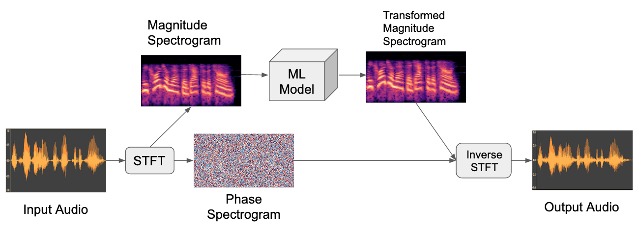
<p>For sequence-to-sequence problems, one strategy is to use the original phase component
of the input signal.</p>

<p><span class="caption">
<img src="/images/loss_functions/reuse_phase.png" alt="Sequence-to-sequence audio modeling in the magnitude spectral domain by re-using the original phase" style="text-align: center;" /><br />
Sequence-to-sequence audio modeling in the magnitude spectral domain by re-using the original phase.
</span></p>

<p>This can work, but it might not sound great for longer sequences that were drastically
transformed by the model.</p>

<p>When that’s not feasible, another option is to come up with a phase component from scratch. This is
the field of research called <strong>phase reconstruction</strong>. One time-tested approach is the <a href="https://paperswithcode.com/method/griffin-lim-algorithm">Griffin-Lim algorithm</a>,
which uses the intuition that the STFT usually results in the same frequencies being
activated in neighboring frames to iteratively come up with a reasonable guess for a phase.</p>

<p>More recently, generative models like the WaveNet[1] and WaveGlow[2] have been used as
“vocoders”, or front-end components that probabilistically generate
waveforms given magnitude spectrograms. You can either add these to your neural net architecture
and train it all end-to-end, or you can use pretrained versions and just focus on training
your custom components.</p>

<p>In recent years it has seemed like generative audio research was heading in
the direction of always modeling the waveform domain end-to-end. However, high quality
vocoders like WaveNet have enabled researchers to continue utilizing the more compact
and in some cases better performing magnitude spectrograms as primary modeling domains.</p>

<p>With that out of the way, onto the loss functions.</p>

<h2 id="l1-and-l2-of-waveforms">L1 and L2 of waveforms</h2>

<p>These are the bread and butter of learning objectives. If you need a reminder:
<strong>L1</strong>, also known as <strong>Mean Absolute Error (MAE)</strong>, involves simply
aligning the two waveforms, finding the absolute difference between each pair of sample points,
and averaging them. <strong>L2</strong>, or <strong>Mean Squared Error (MSE)</strong> is the exact
same except you square each difference before averaging, which has the effect of
penalizing larger errors and being more forgiving of smaller ones.</p>

<p>L1 and L2 are used all the time for audio models in the waveform domain, including
many of the top music source separation approaches [3, 4, 5, 6], and are always worth a try.
However, there are some potential weaknesses to be aware of.</p>

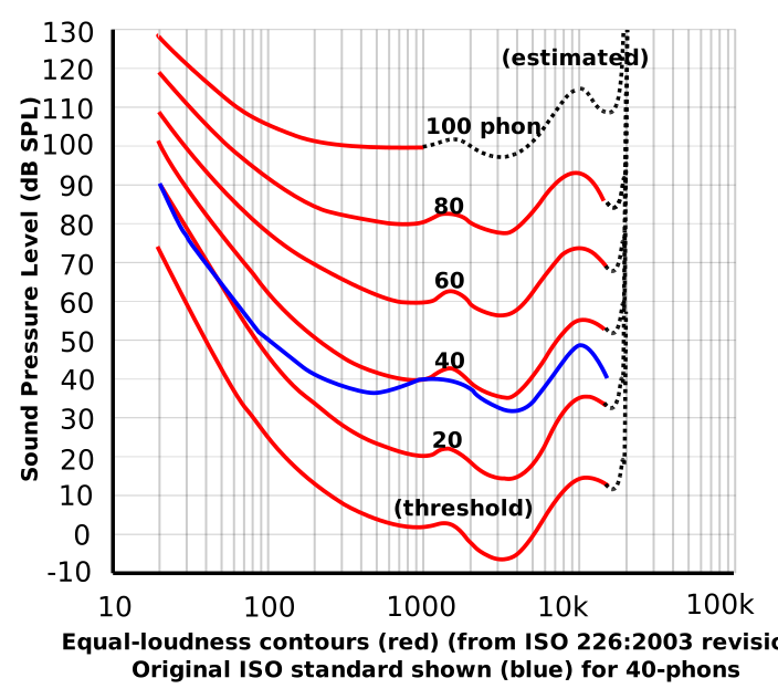
<p>For one, they don’t reflect natural biases in human hearing. Interestingly,
we perceive certain frequencies to be louder or quieter than others, even when they
played with an equal amount of energy. In the 1930’s, researchers actually measured this, resulting in
the first of many “curves” that try to capture human loudness bias as a function of frequency.</p>

<p><span class="caption">
<img src="/images/loss_functions/equal_loudness_contour.svg" alt="Equal-loudness contours (red) (from ISO 226:2003 revision) Original ISO standard shown (blue) for 40-phons" width="512px" /><br />
<a href="https://en.wikipedia.org/wiki/Equal-loudness_contour">Source</a>
</span></p>

<p>If training a model for human ears, with L1/L2 you risk overweighting the
importance of low frequency sounds. One way around this is to use <em>pre-emphasis filters</em>,
which will adjust the energy levels of different frequency channels according to an
equal-loudness curve, such as the one above. <a href="https://librosa.org/doc/main/generated/librosa.effects.preemphasis.html">Librosa</a>
and <a href="https://speechpy.readthedocs.io/en/latest/content/preprocessing.html">SpeechPy</a> offer this functionality.</p>

<p>They also fail to correlate well with human judgement of speech quality and
intelligibility [7].
This makes sense from an evolutionary standpoint – humans had plenty of reasons
to favor our ability to perceive speech, so we evolved neural pathways adept at doing that,
which simpler metrics might not capture.</p>

<h4 id="shift-invariance">Shift Invariance</h4>

<p>Another issue of note is that L1 and L2 in the waveform domain are not shift invariant.
If your models comes up with the exact correct output, but it’s shifted just 1 millisecond
too early or late, a human would consider it a perfect match but error would likely spike.
This can especially manifest as phase shift invariance, where two waves have similar frequencies 
but out-of-sync phases, leading to a large gap in waveform distance.</p>

<p>This might not be a problem for you depending on your goals, or your model of choice.
Recent approaches for sequence-to-sequence problems are converging on the U-Net
architecture, or similar. These models have <a href="https://theaisummer.com/skip-connections/">skip connections</a>,
which are more robust to shift invariance because they have access to the original
input waveform late in the forward pass.</p>

<p>One trick for incorporating shift invariance is <a href="https://en.wikipedia.org/wiki/Dynamic_time_warping">Dynamic Time Warping (DTW)</a>,
whereby dynamic programming is used to find the minimal-cost alignment path between two time series.
This means they can be considered a close match even with mutations or temporal shifts.
A great example can be found in the paper “End-to-End Adversarial Text-to-Speech”[31], where DTW is
used to give the model flexibility on the timing of speech utterances. Note that for
loss functions, you will need to use the differentiable variant <a href="https://github.com/mblondel/soft-dtw">soft-DTW</a>.</p>

<p>Aside from shifts, there are other transformations for which L1/L2 will unfairly penalize.
When it comes to loss functions and evaluation metrics, it’s important to keep in
mind which invariances you care about as a researcher.</p>

<p>Waveform L1/L2 make for great baselines, and it is also common to see them added to other losses.</p>

<h2 id="spectral-losses">Spectral Losses</h2>

<p>Earlier I mentioned how magnitude spectrograms resulting from Fourier transforms offer
a rich data representation, great for both analysis and generation. What I didn’t
mention is that STFT is a differentiable operation!
It should be unsurprising then that L1 and L2 work well as loss functions in the
spectral domain, too. Sometimes you will see this referred to as <strong>spectral loss</strong>,
though there are enough variations that I consider it a family of loss functions.</p>

<p>If your model is already working with spectrograms, then applying L1/L2 is trivial.
But even if it stays in the waveform domain, both tensorflow and pytorch offer
differentiable tensor versions of the STFT that you can apply during training only.</p>

<p>Usually the <em>log</em> magnitude spectrogram is used, sometimes with a small number epsilon added
first, which controls the trade-off between accurately representing low
energy and high energy spectral components [8].</p>

<p style="text-align: center;">$$ \big|\big| log(|STFT(y)| + \epsilon) - log(|STFT(\hat{y})| + \epsilon)\big|\big|_{\ell} $$
<span class="caption">
<b>Log magnitude loss</b>. Here \(y\) is the target signal, \(\hat{y}\) is the predicted, \(||\cdotp||_{\ell}\) is the \(\ell\) norm (like L1 or L2), and \(\epsilon\) is a small number. The absolute value around STFT is a way to discard the phase component.
</span>
</p>

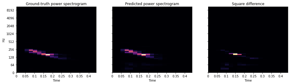
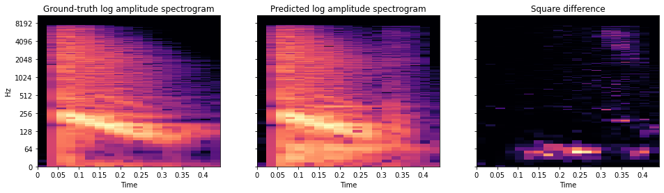
<p><span class="caption">
<img src="/images/loss_functions/spectral_loss.png" alt="Log magnitude spectrogram of a target sound, a prediction from a model, and their squared difference." style="text-align: center;" /><br />
Log magnitude spectrogram of an example sound, a prediction from a model, and their squared difference.
</span></p>

<p>As mentioned previously, STFT involves sliding a window across a waveform, taking
Fourier transforms as you go. This hints at a couple of parameters
that will effect the resulting spectrogram, and thus any downstream learning.
For one, you have to choose a <em>window size</em>. Larger windows will be able to capture
smaller frequencies, but will take up more space. You also need a <em>hop length</em> – it’s common to have successive
windows of samples overlap each other, and hop length in relation to window size determines the extent of this overlap.
In order to minimize the bias of any one choice of parameter, sometimes people use
a <strong>multi-resolution spectral loss</strong> by summing the results of several runs with different window parameters.</p>

<p>Although logarithmic magnitude spectral losses are more common, you do
sometimes see magnitude <em>squared</em>. In signal processing terminology,
this turns <em>amplitude</em> into <em>power</em>, and so you will see this called <strong>power loss</strong>.
As you can see below, a power spectrum concentrates around the strongest frequency bands,
drowning out the others. It follows that power loss is great at ensuring your predictions
have an accurate distribution across the frequency spectrum, in line with your target domain.
For example, it could help a text-to-speech (TTS) system match the highs and lows
of believable human speech [9].</p>

<p><span class="caption">
<img src="/images/loss_functions/spectral_power_loss.png" alt="Power spectrogram of a target sound, a prediction from a model, and their squared difference." style="text-align: center;" /><br />
Power spectrogram of an example sound, a prediction from a model, and their squared difference.
</span></p>

<p>Another related loss you might see is <strong>spectral convergence loss</strong>:</p>

<p style="text-align: center;">$$ \frac{\big|\big| |STFT(y)| - |STFT(\hat{y})| \big|\big|_E}{\big|\big| |STFT(\hat{y})| \big|\big|_E} $$
</p>

<p>\(||\cdotp||_E\) above \(x\) is the Euclidean matrix norm (AKA <a href="https://mathworld.wolfram.com/FrobeniusNorm.html">Frobenius norm</a>).
In words: you take the Euclidean distance of the difference between two magnitude spectrograms,
and normalize it by the Euclidean “length” of the original signal. Similarly to the power
spectrum, since we’re squaring each error component, it highly emphasizes when any one frequency
bucket prediction is way off, and is more forgiving of several frequency bucket predictions being
just a little bit off. According to one paper I read [10], this can especially help in early phases of training.</p>

<h3 id="mel-spectrogram-loss">Mel spectrogram loss</h3>

<p>Earlier I mentioned how humans have natural biases in how we hear loudness at different frequencies.
We also have biases in how we hear pitch. Low frequencies sound “low” to us, and higher
ones sound “high”, but the relationship between frequency and perception is non-linear –
a 100 Hz and 200 Hz sine wave will sound much further apart than a 10,000 Hz and 10,100 Hz wave.
There have been several attempts at codifying this relationship through listening tests;
the most widely used formulation is the <a href="https://en.wikipedia.org/wiki/Mel_scale">Mel scale</a>.
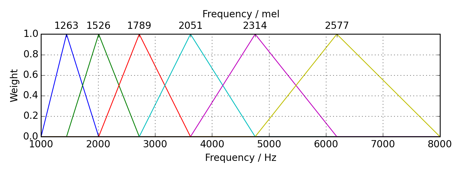
Obtaining the Mel spectrogram is similar to the STFT operation, but frequency energies
are placed into different buckets of equal perceived pitch difference, according to the filterbanks
of the Mel scale.</p>

<p><span class="caption">
<img src="/images/loss_functions/mel_filter_bank.png" alt="The Mel filterbank, showing windows of frequencies that are aggregated into a Mel spectrogram." style="text-align: center;" /><br />
The Mel filterbank, showing windows of frequencies that are aggregated into a Mel spectrogram. <a href="http://siggigue.github.io/pyfilterbank/melbank.html">Source</a>.
</span></p>

<p>Any of the previously mentioned spectral losses can also be carried out using the Mel spectrogram.</p>

<p>A quick side note: the Mel spectrogram is actually a common general representation for modeling audio.
Along with being a better correlate with human pitch perception, it’s also more compact
then normal spectrograms. How much so depends on how precise you make the Mel filterbanks
(e.g. the <code class="language-plaintext highlighter-rouge">n_mels</code> parameter in <a href="https://librosa.org/doc/main/generated/librosa.filters.mel.html#librosa.filters.mel">librosa</a>), but depending on your problem, you can potentially
reduce your space footprint by an order of magnitude without sacrificing performance.
You will, however, need a specialized vocoder model if you want to get back to waveforms from a Mel spectrogram.</p>

<p>Spectral losses come up in many areas, but especially speech enhancement, TTS, and music
synthesis.</p>

<h2 id="source-separation">Source Separation</h2>

<p>Audio source separation is the problem of separating an audio signal into the components (sources)
that were mixed together to create it. One application is in music, where source
separation can be used to “demix” a song (usually into predefined categories, like <code class="language-plaintext highlighter-rouge">bass</code>, <code class="language-plaintext highlighter-rouge">drums</code>,
<code class="language-plaintext highlighter-rouge">vocals</code>, and <code class="language-plaintext highlighter-rouge">other</code>). Another application is voice separation,
which attempts to tackle the classic <a href="https://en.wikipedia.org/wiki/Cocktail_party_effect">cocktail party problem</a>
by isolating individual voices from a conversation, or from the background of a recording.</p>

<p>During model training, each predicted source is compared to a ground truth target using an
objective function. While the losses covered above can work just fine, another is more
common. For the following, suppose you are trying to predict the source signal \(s\),
and your model comes up with an imperfect \(\hat{s}\).</p>

<p><strong>SDR (Source to Distortion Ratio):</strong></p>

\[SDR := 10 \cdot log_{10}\frac{||s||^2}{||s - \hat{s}||^2}\]

<p>This metric is measured in <a href="https://en.wikipedia.org/wiki/Sound_pressure#Sound_pressure_level">decibels</a>,
where higher is better. Any mistake in the prediction will cause the denominator to grow,
which will cause the overall metric to go down.</p>

<p>SDR is equivalent to the classic <a href="https://en.wikipedia.org/wiki/Signal-to-noise_ratio">signal-to-noise ratio</a>,
so sometimes you will see it reported as SNR. However, there is a totally different
SNR metric (Sources to Noise Ratio) also sometimes used to evaluate source separation results,
so be careful to know which one you’re dealing with.</p>

<h4 id="scale-invariance">Scale invariance</h4>

<p>A major downside of vanilla SDR is that it’s sensitive to the loudness of the predicted
signal. If you were to scale the prediction up or down, the metric would rise
or fall along a curve around some point of “ideal” scale. In the context of SDR
as an evaluation metric, this means some researchers might optimize scale to achieve
the highest score and others might not, leading to unfair comparisons. In the context
of SDR as an objective function, I think this would lead to a slower and less-smooth
learning curve.</p>

<p>Thankfully, some researchers <a href="https://arxiv.org/abs/1811.02508">surfaced</a> the issue
in 2018 and came up with a scale-invariant version of SDR where the optimal
scaling factor is baked in.</p>

<p><strong>SI-SDR (Scale-Invariant Source to Distortion Ratio):</strong></p>

\[SI-SDR := 10 \cdot log_{10}\Bigg(\frac{||\frac{\hat{s}^Ts}{||s||^2} s||^2}{||\frac{\hat{s}^Ts}{||s||^2} s - \hat{s}||^2}\Bigg)\]

<p>Again, sometimes you will see this reported as <code class="language-plaintext highlighter-rouge">SI-SNR</code>. At this point, I see no reason why anyone would want to use plain SDR in favor of
the scale-invariant version.</p>

<h4 id="permutation-invariance">Permutation invariance</h4>

<p>When you know the categories of sources ahead of time and your training set comes with
labeled sources, you can just add the losses from each prediction. However, for problems
with an unknown number of sources (called <em>blind source separation</em>), such as in the cocktail party problem,
it’s not that simple. You need to know <em>which</em> predictions correspond to which ground
truth targets. Further, you’ll want a one-to-one correspondence between the predictions
and targets, so that you don’t end up with two predictions of the same source or
not enough predicted sources. Using random assignments at every optimization step
would unfairly penalize the model for a bad roll of the dice, leading to very unstable
training. Rather, in these cases you should apply your loss function in a
permutation invariant way. One such method is <strong>Permutation Invariant Training (PIT)</strong>,
wherein every combination of assignments is attempted, and the best set
(lowest combined loss) is used. This incentivizes the model to settle into learning
each source once, without needing to care in what order they are output.</p>

<p>The <code class="language-plaintext highlighter-rouge">asteroid</code> library offers a <a href="https://asteroid-team.github.io/asteroid/package_reference/losses.html#permutation-invariant-training-pit-made-easy">wrapper Python class</a>
that makes it easy to turn any loss function into a permutation-invariant version.</p>

<h2 id="perceptual-loss">Perceptual Loss</h2>

<p>Neural networks are great at discovering features that distinguish between inputs.
And it’s often easy to imagine other problems for which the same features would be helpful.
For example, a facial recognition model might have a neuron that
fires when presented with a horizontal line, which might be used by a higher-level
neuron to decide whether the picture contains a chin. If you were then designing a
person-detection model, it could probably benefit from being able to detect both chins and faces.</p>

<p>So how could you utilize features from a network trained to solve problem \(A\)
to help train a network to solve a similar problem \(B\)? This is the research area
known as <a href="https://ruder.io/transfer-learning/">transfer learning</a>. The simplest way is
to directly feed the feature values into your new network. In our example above, the
person-detection network would see its normal inputs, but would <em>also</em> be given the neuron
values from the facial detection network to work with. Another way is <em>fine-tuning</em>,
where network \(A\) is first trained to solve problem \(A\), and then further trained
to solve problem \(B\).</p>

<p>Neural features are not just numbers; they are connected to other neurons, that,
once fully unrolled, are large differentiable functions. We should be able to
utilize these function gradients without being forced to re-use the neural architecture
of network \(A\) to solve problem \(B\). These are the insights that motivate <strong>perceptual loss</strong>,
also known as <strong>deep feature loss</strong>. Perceptual loss was inspired by research on <a href="https://www.cv-foundation.org/openaccess/content_cvpr_2016/papers/Gatys_Image_Style_Transfer_CVPR_2016_paper.pdf">style transfer</a> in computer
vision.</p>

<p>Lets assume you have already trained an auxiliary task \(B\) (seen in the figure below
in red). The basic idea is to use the features of \(B\) to compute a gradient that updates \(A\) in a
way that makes audio predicted by \(A\) closer to ground-truth audio <em>in \(B\)’s feature space</em>.
Usually in deep learning the parameters being updated during optimization are the
same ones that were used to compute the gradient. However, here \(B’s\) parameters
are frozen.</p>

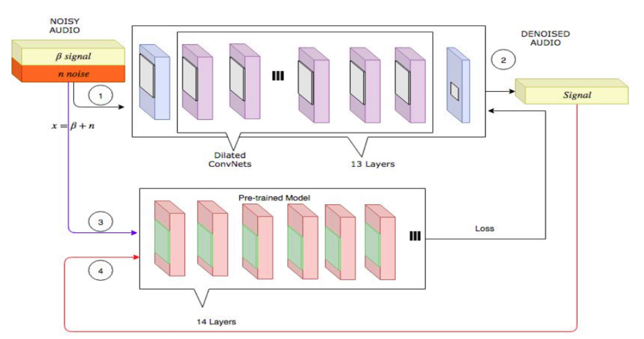
<p><span class="caption">
<img src="/images/loss_functions/perceptual_loss.png" alt="A depiction of perceptual loss learning in the audio denoising domain." style="text-align: center;" /><br />
A depiction of perceptual loss learning in the audio denoising domain. First a batch
of training inputs is put through the network being optimized (top). The output is then put
through an auxiliary network (bottom), pre-trained on a similar problem. Finally, the original
batch of signals is also put through the auxiliary network, and the two activations
are compared to compute a gradient that updates the original network. <a href="https://labs.imaginea.com/shabda-a-neural-speech-denoiser/">Source</a>.
</span></p>

<p>The loss formula is usually something called <em>feature reconstruction loss</em>, where you sum
the L1/L2 distances of neural activations of the auxiliary network’s first \(k\) layers.
Using earlier layers favors reusable patterns over high-level features
that tend to be specific to the auxiliary task.</p>

<p>Here are some examples from audio research:</p>
<ul>
  <li>“Parallel wavenet: Fast high-fidelity speech synthesis”[9] – among other loss components,
they include a perceptual loss term using a network trained to detect the phonemes of
speech signals. They basically utilize speech-to-text features as a means
of improving text-to-speech, which I find to be an interesting parrallel.</li>
  <li>“Voice Separation with an Unknown Number of Multiple Speakers”[11] – they attempt the
cocktail party problem using perceptual loss against a networked trained on speaker identification.
The intuition is that if a network is able to pick apart the nuances of different speakers’ voices,
it should also provide useful features for separating voices from background audio.</li>
  <li>“Hierarchical Timbre-Painting and Articulation Generation”[12] – they attempt a kind of
music synthesis whereby you take a source recording of some instrument playing a melody,
and render it as a completely different instrument, while preserving the nuances
of pitch and loudness. Their auxiliary network of choice is the pitch-detecting <a href="https://arxiv.org/abs/1802.06182">CREPE</a>, with
some <a href="https://mosheman5.github.io/timbre_painting/">pretty cool results here</a>.</li>
  <li>“Deep Network Perceptual Losses For Speech Denoising”[13] – they utilize a deep feature loss
based on speech detection as an auxiliary task, as well as one trained on the audio
event detection dataset <a href="http://research.google.com/audioset/">AudioSet</a>.</li>
</ul>

<h2 id="learned-perceptual-loss">Learned Perceptual Loss</h2>

<p>In the search for a metric that highly correlates with human perception, the authors of
“A Differentiable Perceptual Audio Metric Learned from Just Noticeable Differences”[14]
take a unique approach.</p>

<p>They first crowdsource a dataset of human judgements that capture “just noticeable differences” (JND) – users are presented
with two audio recordings, where one is a slightly perturbed version of the other,
and asked whether they are exactly the same sounds or not. The amount of perturbation
(e.g. reverb, compression, dropouts) is carefully chosen to be small enough so that the
authors end up with lots of data right around the threshold of what’s barely noticeable.</p>

<p>They then fit a deep neural network to predict these human judgements, by minimizing
binary cross-entropy. The resulting network can be used as a quality metric, and, since
it is differentiable, as a learning objective (similarly to how you would use the perceptual losses above).
They call their metric DPAM, available for both <a href="https://github.com/pranaymanocha/PerceptualAudio">tensorflow</a>
and <a href="https://github.com/adrienchaton/PerceptualAudio_pytorch">pytorch</a>. More recently they
released an improved metric called CDPAM[15], which is more
robust to perturbations not used in the original JND dataset.</p>

<p>The released version of CDPAM is meant to be general-purpose, but their approach
also seems quite adaptable. If you have particular requirements for your ideal similarity metric,
or you’re working in a specialized domain with access to a pool of experts, you should
be able to capture your requirements in a JND dataset and train a metric yourself.</p>

<h2 id="other">Other</h2>

<h3 id="speech-quality-metrics">Speech Quality Metrics</h3>

<p>If you work in speech enhancement or TTS, you may come across the metric <a href="https://en.wikipedia.org/wiki/Perceptual_Evaluation_of_Speech_Quality">PESQ</a>. Originally a commercial telecomm specification,
it is differentiable, but only defined up to frequencies of 8k so not ideal for learning [16].
It did inspire a newer trainable variant PMSQE[17], which looks promising.</p>

<p>You may also come across Short-Time Objective Intelligibility (STOI)[18], which is differentiable
but usually just used as an evaluation metric.</p>

<h3 id="categorical-cross-entropy">Categorical cross entropy</h3>

<p>You might not have expected to see a categorical loss for inherently continuous waveform data.
Nonetheless, architectures like WaveNet[1] model waveform sample probabilities as discrete classes
under a softmax distribution.</p>

<p>One benefit of quantization is that it prevents mode collapse. Sometimes models predicting
continuous-valued waveforms will cut their losses by mostly just outputting the safest
option between -1 and 1: zero (or near it). This is especially true earlier in the
training process. By instead predicting non-ordinal classes, no such safe option exists
and the model is forced into trying <em>something</em>.</p>

<h2 id="conclusion">Conclusion</h2>

<p>During my informal survey of research from the past five years or so, I noticed some trends:</p>

<table>
  <thead>
    <tr>
      <th style="text-align: left">In…</th>
      <th style="text-align: center">They tend to use…</th>
    </tr>
  </thead>
  <tbody>
    <tr>
      <td style="text-align: left">Music Source Separation</td>
      <td style="text-align: center">L1/L2 of waveforms [3][4][5][6]</td>
    </tr>
    <tr>
      <td style="text-align: left">Speech Separation</td>
      <td style="text-align: center">SI-SDR [11][19][20][21]</td>
    </tr>
    <tr>
      <td style="text-align: left">Voice Conversion</td>
      <td style="text-align: center">L1/L2 in Mel spectral domain, adversarial losses [22][23][24]</td>
    </tr>
    <tr>
      <td style="text-align: left">Text-to-speech</td>
      <td style="text-align: center">L1/L2 in spectral domains, especially Mel [25][26][27][28][29][30]</td>
    </tr>
  </tbody>
</table>

<p>These are not endorsements, just patterns. Other areas had no clear consensus. Here are some additional tips for practitioners:</p>
<ul>
  <li>Start with L1 in whichever domain is easiest given your model architecture, then expand your search.</li>
  <li>Don’t be afraid to mix several loss functions. It’s not uncommon to see three or even four components.</li>
  <li>Strive to use as many evaluation metrics as you can. Be especially careful if you’re using the
same metric for both an objective function <em>and</em> evaluation, as it may leave you thinking
your model is performing better than it actually is.</li>
</ul>

<p>If you’re using pyTorch and looking to try some of these out, I recommend the <a href="https://github.com/csteinmetz1/auraloss">auraloss</a>
library, or <a href="https://asteroid-team.github.io/asteroid/package_reference/losses.html">asteroid</a>
if you’re working on source/voice separation. Sadly I could not find anything similar
for tensorflow (any readers in need of a side project?…)</p>

<p>There are many objective functions available for your audio models, and given the number of
potential combinations, you may not be able to try them all. By being informed
about their pros, cons, and prevalences, I hope you can save precious GPU hours.</p>

<p><br /></p>

<div class="ad">
  <div class="ad-column-left">
    <p>
      <p>Have some data and a problem to solve?</p>
      <p>I'm available for consulting and contract work.</p>
      <p><a href="/consulting">Learn more</a></p>
    </p>
  </div>
  <div class="ad-column-right">
    <div class="icon-container">
      <a href="mailto:evan@soundsandwords.io">
        <i class="svg-icon-large email-large"></i>
      </a>
    </div>
  </div>
</div>

<h4 id="references">References</h4>

<ul class="bib">
  <li>[1] A. Oord. WaveNet: A generative model for raw audio, 2016.</li>
  <li>[2] R. Prenger. WaveGlow: a Flow-based Generative Network for Speech Synthesis, 2018.</li>
  <li>[3] A. Défossez. Music Source Separation in the Waveform Domain, 2019.</li>
  <li>[4] D. Stoller. Wave-U-Net: A Multi-Scale Neural Network for End-to-End Audio Source Separation, 2018.</li>
  <li>[5] R. Hennequin. Spleeter: a Fast and Efficient Music Source Separation Tool with Pre-Trained Models, 2020.</li>
  <li>[6] N. Takahashi. D3Net: Densely connected multidilated DenseNet for music source separation, 2020.</li>
  <li>[7] S. Fu. MetricGAN+: An Improved Version of MetricGAN for Speech Enhancement, 2021.</li>
  <li>[8] A. Défossez. SING: Symbol-to-Instrument Neural Generator, 2018.</li>
  <li>[9] A. Oord. Parallel WaveNet: Fast High-Fidelity Speech Synthesis, 2017.</li>
  <li>[10] S. Arik. Fast Spectrogram Inversion using Multi-head Convolutional Neural Networks, 2018.</li>
  <li>[11] E. Nachmani. Voice Separation with an Unknown Number of Multiple Speakers, 2020.</li>
  <li>[12] M. Michelashvili. Hierarchical Timbre-Painting and Articulation Generation, 2020.</li>
  <li>[13] M. Saddler. Deep Network Perceptual Losses For Speech Denoising, 2020.</li>
  <li>[14] P. Manocha. A Differentiable Perceptual Audio Metric Learned from Just Noticeable Differences, 2020.</li>
  <li>[15] P. Manocha. CDPAM: Contrastive learning for perceptual audio similarity, 2021.</li>
  <li>[16] <a href="https://operata.com/blog/polqa-vs-pesq">POLQA Vs PESQ: Objective quality scoring explained</a>.</li>
  <li>[17] J. Martín-Doñas. A Deep Learning Loss Function based on the Perceptual Evaluation of the Speech Quality, 2019.</li>
  <li>[18] C. Taal. A short-time objective intelligibility measure for time-frequency weighted noisy speech, 2010.</li>
  <li>[19] Y. Luo. Conv-TasNet: Surpassing Ideal Time-Frequency Magnitude Masking for Speech Separation, 2019.</li>
  <li>[20] C. Subakan. Attention is All You Need in Speech Separation, 2020.</li>
  <li>[21] M. Pariente. Filterbank design for end-to-end speech separation, 2019.</li>
  <li>[22] H. Kameoka. StarGAN-VC: Non-parallel many-to-many voice conversion with star generative adversarial networks, 2018.</li>
  <li>[23] S. Wang. NoiseVC: Towards High Quality Zero-Shot Voice Conversion, 2021.</li>
  <li>[24] J. Zhang. Sequence-to-Sequence Acoustic Modeling for Voice Conversion, 2018.</li>
  <li>[25] Y. Wang. Tacotron: Towards End-to-End Speech Synthesis, 2017.</li>
  <li>[26] J. Shen. Natural TTS Synthesis by Conditioning WaveNet on Mel Spectrogram Predictions, 2017.</li>
  <li>[27] Y. Jia. Transfer Learning from Speaker Verification to Multispeaker Text-To-Speech Synthesis, 2018.</li>
  <li>[28] A. Gritsenko. A Spectral Energy Distance for Parallel Speech Synthesis, 2020.</li>
  <li>[29] X. Wang. Neural source-filter-based waveform model for statistical parametric speech synthesis, 2018.</li>
  <li>[30] W. Ping. Deep Voice 3: Scaling Text-to-Speech with Convolutional Sequence Learning, 2017.</li>
  <li>[31] J. Donahue. End-to-End Adversarial Text-to-Speech, 2021.</li>
</ul>]]></content><author><name>Evan Radkoff</name></author><category term="Sounds" /><category term="Loss Functions" /><category term="Objective Functions" /><summary type="html"><![CDATA[An informal survey of objective functions used in Machine Learning in the audio domain.]]></summary><media:thumbnail xmlns:media="http://search.yahoo.com/mrss/" url="https://soundsandwords.io//images/loss_functions/spectral_loss.png" /><media:content medium="image" url="https://soundsandwords.io//images/loss_functions/spectral_loss.png" xmlns:media="http://search.yahoo.com/mrss/" /></entry><entry><title type="html">3 Ways to Classify Drum Sounds</title><link href="https://soundsandwords.io//drum-sound-classification/" rel="alternate" type="text/html" title="3 Ways to Classify Drum Sounds" /><published>2020-11-29T00:00:00+00:00</published><updated>2020-11-29T00:00:00+00:00</updated><id>https://soundsandwords.io//drum-sound-classification</id><content type="html" xml:base="https://soundsandwords.io//drum-sound-classification/"><![CDATA[<p>Drums libraries have been one of the most important developments in digital music production. We’re no longer restricted to the stock sounds that come with drum machines, allowing for more room to develop a unique sound. We’ve seen a surge in free drum kits on the web, and there’s an ever-growing list of digital audio workstations with which to use them.</p>

<p>As my own drum library has exploded in size (ok I’m a hoarder), it’s got me thinking of ways to take control and organize it better. One thing that has bugged me is the inconsistent naming of sound files:</p>
<ul>
  <li>Abbreviations like <code class="language-plaintext highlighter-rouge">CR.wav</code> for a crash cymbal, that wouldn’t come up in a search</li>
  <li>Different classification schemes, e.g. <code class="language-plaintext highlighter-rouge">Perc.wav</code> for ‘percussion’, instead of something more specific like rimshot</li>
  <li>Labels I don’t agree with, or are just flat out wrong</li>
</ul>

<p>It would help to have my own way of assigning drum sound labels, and in this post I will share several ways to achieve that with ML.</p>

<blockquote>
  <p>All code is <a href="https://github.com/radkoff/drum_sound_classifier">open-source</a>, so you can follow along and try this out yourself! You only need python and your own <a href="https://reddit.com/r/drumkits">drum sounds</a>.</p>
</blockquote>

<h2 id="what-do-drum-sounds-look-like">What do drum sounds look like?</h2>
<p>If you’ve ever worked with audio data you’re probably familiar with waveforms, which show the raw signals that might be sent to speakers for playback. Spectrograms are more insightful because they separate a signal into different frequency bands, allowing you to see the amount of energy up and down the spectrum. See examples of both below.</p>

<h4 id="snares">Snares</h4>

<p><img src="/images/drum_sound_classification/snare.jpg" alt="Waveforms and spectrograms of a few random snare sounds" style="width: 800px; text-align: center;" /></p>

<h4 id="kicks">Kicks</h4>
<p><img src="/images/drum_sound_classification/kick.jpg" alt="Waveforms and spectrograms of a few random kick sounds" style="width: 800px; text-align: center;" /></p>

<h4 id="toms">Toms</h4>
<p><img src="/images/drum_sound_classification/tom.jpg" alt="Waveforms and spectrograms of a few random tom sounds" style="width: 800px; text-align: center;" /></p>

<p style="font-size: 9pt; text-align: center;">Plots above made with <a href="https://librosa.org/">librosa</a>, a great python library for audio processing.</p>

<p>You’ll notice some patterns, like how the snare waveforms look “fuzzier” and have energy up and down the spectrum. Kicks are obviously strongest in the lower frequencies (you can see spikes around 64 Hz), and toms look similar to kicks in ways but have spikes anywhere from 100Hz-500Hz. Now, lets see what ML can do.</p>

<h2 id="a-taxonomy">A taxonomy</h2>

<p>I needed a set of drum type classes. A few options came up in research, the simplest being <code class="language-plaintext highlighter-rouge">bass drum, snare drum, hi-hat</code> (used in <a href="https://dumas.ccsd.cnrs.fr/ENST/pastel-00002805">this thesis</a> and elsewhere). A limited set like that would make prediction easy, but it’s not as useful. The authors of <a href="https://citeseerx.ist.psu.edu/viewdoc/download?doi=10.1.1.18.5451&amp;rep=rep1&amp;type=pdf">one paper</a> used a scheme closer to that of a standard rock kit: <code class="language-plaintext highlighter-rouge">kick, snare, low tom, medium tom, high tom, open hi-hat, closed hi-hat, ride, crash</code>. There’s even the <a href="https://en.wikipedia.org/wiki/General_MIDI#Program_change_events">General MIDI spec</a> with dozens of percussive types – though, with that many classes it becomes hard to build up a dataset with enough of each.</p>

<p>I wanted to strike the right balance of taxonomy size, while also choosing classes more reflective of modern hip-hop and electronic drum kits found on the web. So, I made my own: <code class="language-plaintext highlighter-rouge">hat, tom, ride [cymbal], open [hi-hat], kick, bongo [and conga], clap, snare, rim, snap, crash [cymbal], shaker</code></p>

<h2 id="building-a-clean-dataset">Building a clean dataset</h2>

<p>Drum libraries are usually scattered across different folders, so given the top-level folder, it shouldn’t be hard to recursively walk and find all eligible sounds. I’m a fan of using <a href="https://pandas.pydata.org/">pandas</a> to explore data, so I initialized a DataFrame with one sound per row.</p>

<div class="language-python highlighter-rouge"><div class="highlight"><pre class="highlight"><code><span class="k">def</span> <span class="nf">read_drum_library</span><span class="p">(</span><span class="n">input_dir_path</span><span class="p">):</span>
    <span class="n">logger</span><span class="p">.</span><span class="nf">info</span><span class="p">(</span><span class="sa">f</span><span class="sh">'</span><span class="s">Searching for audio files found in </span><span class="si">{</span><span class="n">input_dir_path</span><span class="si">}</span><span class="sh">'</span><span class="p">)</span>

    <span class="n">dataframe_rows</span> <span class="o">=</span> <span class="p">[]</span>
    <span class="k">for</span> <span class="n">input_file</span> <span class="ow">in</span> <span class="n">input_dir_path</span><span class="p">.</span><span class="nf">glob</span><span class="p">(</span><span class="sh">'</span><span class="s">**/*.*</span><span class="sh">'</span><span class="p">):</span>
        <span class="n">absolute_path_name</span> <span class="o">=</span> <span class="n">input_file</span><span class="p">.</span><span class="nf">resolve</span><span class="p">().</span><span class="nf">as_posix</span><span class="p">()</span>
        <span class="k">if</span> <span class="ow">not</span> <span class="nf">can_load_audio</span><span class="p">(</span><span class="n">absolute_path_name</span><span class="p">):</span>
            <span class="k">continue</span>

        <span class="n">properties</span> <span class="o">=</span> <span class="p">{</span>
            <span class="sh">'</span><span class="s">audio_path</span><span class="sh">'</span><span class="p">:</span> <span class="n">absolute_path_name</span><span class="p">,</span>
            <span class="sh">'</span><span class="s">store_path</span><span class="sh">'</span><span class="p">:</span> <span class="n">file_store_path</span><span class="p">.</span><span class="nf">as_posix</span><span class="p">(),</span>
            <span class="sh">'</span><span class="s">file_stem</span><span class="sh">'</span><span class="p">:</span> <span class="nc">Path</span><span class="p">(</span><span class="n">absolute_path_name</span><span class="p">).</span><span class="n">stem</span><span class="p">.</span><span class="nf">lower</span><span class="p">(),</span>
            <span class="sh">'</span><span class="s">start_time</span><span class="sh">'</span><span class="p">:</span> <span class="mf">0.0</span><span class="p">,</span>
            <span class="sh">'</span><span class="s">end_time</span><span class="sh">'</span><span class="p">:</span> <span class="n">np</span><span class="p">.</span><span class="n">NaN</span>
        <span class="p">}</span>
        <span class="c1"># Tack on the original file duration (will have to load audio)
</span>        <span class="n">audio</span> <span class="o">=</span> <span class="n">read_audio</span><span class="p">.</span><span class="nf">load_raw_audio</span><span class="p">(</span><span class="n">absolute_path_name</span><span class="p">,</span> <span class="n">fast</span><span class="o">=</span><span class="bp">True</span><span class="p">)</span>
        <span class="n">properties</span><span class="p">[</span><span class="sh">'</span><span class="s">orig_duration</span><span class="sh">'</span><span class="p">]</span> <span class="o">=</span> <span class="nf">len</span><span class="p">(</span><span class="n">audio</span><span class="p">)</span> <span class="o">/</span> <span class="nf">float</span><span class="p">(</span><span class="n">read_audio</span><span class="p">.</span><span class="n">DEFAULT_SR</span><span class="p">)</span>

        <span class="n">dataframe_rows</span><span class="p">.</span><span class="nf">append</span><span class="p">(</span><span class="n">properties</span><span class="p">)</span>

    <span class="k">return</span> <span class="n">pandas</span><span class="p">.</span><span class="nc">DataFrame</span><span class="p">(</span><span class="n">dataframe_rows</span><span class="p">)</span>
</code></pre></div></div>

<p>I got rid of really quiet sounds by thresholding <a href="https://musicinformationretrieval.com/energy.html">RMS</a>, and also excluded those over 5 seconds.</p>

<p>I wanted to go even further in isolating single percussive hits, because I had noticed some loops with multiple hits that might throw off a model. I also wanted some consistency around how much silence appeared at the begging of sounds. My solution for both of these issues was to use <code class="language-plaintext highlighter-rouge">librosa</code>’s onset detection API. An <a href="https://musicinformationretrieval.com/onset_detection.html">onset</a> is the moment that marks the beginning of a rise in energy of a sound. All I had to do is set the start time of each sound to just before the first onset, and the end time to just before any second onset.</p>

<p>One downside of the supervised deep learning techniques we’ll see later is that they require a lot of data. It’s easy to find tons of drum kits on the web, but what about labels? Fortunately, we can build up a dataset without manual annotations by just trusting the original filenames. They won’t be perfect, but they’ll be good enough to start.</p>

<div class="language-python highlighter-rouge"><div class="highlight"><pre class="highlight"><code><span class="n">DRUM_TYPES</span> <span class="o">=</span> <span class="p">[</span><span class="sh">'</span><span class="s">hat</span><span class="sh">'</span><span class="p">,</span> <span class="sh">'</span><span class="s">tom</span><span class="sh">'</span><span class="p">,</span> <span class="sh">'</span><span class="s">ride</span><span class="sh">'</span><span class="p">,</span> <span class="sh">'</span><span class="s">open</span><span class="sh">'</span><span class="p">,</span> <span class="sh">'</span><span class="s">kick</span><span class="sh">'</span><span class="p">,</span> <span class="sh">'</span><span class="s">bongo</span><span class="sh">'</span><span class="p">,</span> <span class="sh">'</span><span class="s">clap</span><span class="sh">'</span><span class="p">,</span> <span class="sh">'</span><span class="s">snare</span><span class="sh">'</span><span class="p">,</span> <span class="sh">'</span><span class="s">rim</span><span class="sh">'</span><span class="p">,</span> <span class="sh">'</span><span class="s">snap</span><span class="sh">'</span><span class="p">,</span> <span class="sh">'</span><span class="s">crash</span><span class="sh">'</span><span class="p">,</span> <span class="sh">'</span><span class="s">shaker</span><span class="sh">'</span><span class="p">]</span>
<span class="n">drums_df</span> <span class="o">=</span> <span class="nf">read_drum_library</span><span class="p">(</span><span class="n">drum_lib_path</span><span class="p">)</span>
<span class="k">for</span> <span class="n">drum_type_class</span> <span class="ow">in</span> <span class="n">DRUM_TYPES</span><span class="p">:</span>
    <span class="n">drum_sounds</span><span class="p">.</span><span class="n">loc</span><span class="p">[</span><span class="n">drum_sounds</span><span class="p">.</span><span class="n">file_stem</span><span class="p">.</span><span class="nb">str</span><span class="p">.</span><span class="nf">contains</span><span class="p">(</span><span class="n">drum_type_class</span><span class="p">),</span> <span class="sh">'</span><span class="s">file_drum_type</span><span class="sh">'</span><span class="p">]</span> <span class="o">=</span> <span class="n">drum_type_class</span>
</code></pre></div></div>

<blockquote>
  <p>If you’re following along <a href="https://github.com/radkoff/drum_sound_classifier">at home</a>, you can run:</p>
  <div class="language-shell highlighter-rouge"><div class="highlight"><pre class="highlight"><code>python preprocess.py <span class="nt">--drum_lib_path</span> ~/Music/drums
</code></pre></div>  </div>
</blockquote>

<p>With that, my dataset looked like this:</p>

<div class="language-shell highlighter-rouge"><div class="highlight"><pre class="highlight"><code><span class="o">&gt;</span> import pickle
<span class="o">&gt;</span> drums <span class="o">=</span> pickle.load<span class="o">(</span>open<span class="o">(</span><span class="s1">'data/interim/dataset.pkl'</span>, <span class="s1">'rb'</span><span class="o">))</span>
<span class="o">&gt;</span> drums <span class="o">=</span> drums[~drums.file_drum_type.isna<span class="o">()]</span>   <span class="c"># Restrict to sounds with recognizable file labels</span>
<span class="o">&gt;</span> drums.info<span class="o">()</span>
Data columns <span class="o">(</span>total 7 columns<span class="o">)</span>:
 <span class="c">#   Column          Non-Null Count     Dtype  </span>
<span class="nt">---</span>  <span class="nt">------</span>          <span class="nt">--------------</span>     <span class="nt">-----</span>  
 0   audio_path      11672 non-null     object
 1   store_path      11672 non-null     object
 2   file_stem       11672 non-null     object
 3   start_time      11672 non-null     float64
 4   end_time        818   non-null     float64
 5   orig_duration   11672 non-null     float64
 6   file_drum_type  11672 non-null     object
dtypes: float64<span class="o">(</span>3<span class="o">)</span>, object<span class="o">(</span>4<span class="o">)</span>
memory usage: 1.2+ MB

<span class="o">&gt;</span> drums[[<span class="s1">'file_stem'</span>, <span class="s1">'start_time'</span>, <span class="s1">'end_time'</span>, <span class="s1">'file_drum_type'</span><span class="o">]]</span>.sample<span class="o">(</span>5<span class="o">)</span>
   file_stem  start_time  end_time file_drum_type
15   openhat    0.000000       NaN           open
5     kick18    0.000000       NaN           kick
38   schat13    0.000000       NaN            hat
2    lakick9    0.000000       NaN           kick
19    kick8     0.022653  0.092494           kick

<span class="o">&gt;</span> drums.drum_type.value_counts<span class="o">()</span>
snare     2952
kick      2845
hat       1805
tom       1371
clap      1048
rim        436
open       337
ride       263
crash      257
snap       110
bongo      101
shaker      98
</code></pre></div></div>

<p>As you can see, I had a pretty large class imbalance. This can be bad for model performance on the lesser represented classes. One way to help with this is over-sampling via something like <a href="https://github.com/scikit-learn-contrib/imbalanced-learn">imbalanced-learn</a> or pyTorch’s <code class="language-plaintext highlighter-rouge">WeightedRandomSampler</code>. Instead, during training procedures I simply capped class size at 2000 like so:</p>

<div class="language-python highlighter-rouge"><div class="highlight"><pre class="highlight"><code><span class="n">drums</span> <span class="o">=</span> <span class="n">drums</span><span class="p">.</span><span class="nf">groupby</span><span class="p">(</span><span class="sh">'</span><span class="s">file_drum_type</span><span class="sh">'</span><span class="p">).</span><span class="nf">head</span><span class="p">(</span><span class="mi">2000</span><span class="p">)</span>
</code></pre></div></div>

<h2 id="method-1-hand-crafted-features--random-forest">Method 1: Hand-crafted Features + Random Forest</h2>

<p>Analyzing percussion sounds is not new. Let’s look at some of the hand-crafted features that have been used in the past. First, a few from the MPEG-7 standards that reflect the change in a signal’s power over time:</p>

<ul>
  <li>Log attack time - “attack” here means how quickly the signal reaches its peak.</li>
  <li>Temporal centroid - this measures how far along into the sound we’ve reached half of the signal’s power. A sound that starts loud and fades will have an early temporal centroid, while something like a crash cymbal will have a later one.</li>
  <li>Spectral centroid - similarly, this measures the center of gravity in the frequency domain. You can think of it as how low or high the sound is. Since it changes over the duration of the signal, we’ll take the average.</li>
</ul>

<p>Since we’re using “attack”, we can also include “release”, which measures how long the signal lasts from its peak before dipping below a threshold (I use 2% of the peak, following the lead of <a href="https://staff.aist.go.jp/m.goto/PAPER/IEEETASLP200802pampalk.pdf">this paper</a>). There are also other spectral features we can utilize, many provided by <code class="language-plaintext highlighter-rouge">librosa</code>:</p>

<ul>
  <li><a href="https://librosa.org/doc/latest/generated/librosa.feature.spectral_bandwidth.html">Spectral bandwidth</a> - Intuitively, how spread out the frequency spectrum is. Technically, the second central moment of the spectrum.</li>
  <li><a href="https://librosa.org/doc/latest/generated/librosa.feature.spectral_flatness.html">Spectral flatness</a> - measures how noise-like a sound is, as opposed to an isolated tone</li>
  <li><a href="https://librosa.org/doc/latest/generated/librosa.feature.spectral_rolloff.html">Spectral rolloff</a> - as opposed to the spectral centroid, this measures at what frequency a certain percentage of the magnitude distribution is less than. To capture the low and high ends of the frequency spectrum, we’ll compute the rolloff at 15% and 85%.</li>
</ul>

<p>Some additional features we can pull in:</p>

<ul>
  <li>Duration</li>
  <li>Average, max, and standard deviation of log RMS - RMS is root mean squared energy, which you can just think of as volume for our purposes.</li>
  <li>Average change in RMS - since we compute RMS per <em>frame</em> of audio (each frame is ~23 ms in my implementation), we can also look at how it goes up and down between frames. This is also true for other features in this list.</li>
  <li>Crest factor - measures how intense the audio’s peaks are. Peak RMS divided by  average RMS.</li>
  <li><a href="https://librosa.org/doc/latest/generated/librosa.feature.zero_crossing_rate.html">Zero crossing rate</a> (ZCR) - If you zoom in on a waveform, you’ll see the signal oscillating above and below zero. This measures how many times that happens in one frame of audio. We can take the average across all frames, the standard deviation, or the ZCR at the loudest frame since that’s probably revealing.</li>
</ul>

<p>One last set of features worth consideration is the Mel Frequency Cepstral Coefficients (MFCCs). If you hear multiple instruments playing a note at the exact same pitch and volume, you will probably still be able to tell them apart. This is because they exhibit different “timbre” characteristics. MFCCs are a set of (typically 10-20) features great at capturing timbre. I found a great explanation in <a href="https://haythamfayek.com/2016/04/21/speech-processing-for-machine-learning.html">another blog</a>.</p>

<p>After applying summary statistics (average, max, standard deviation, ZCR, and derivative) to frame-based features, I ended up with 72 features in total.</p>

<p>There were some missing values from when I couldn’t take the derivative of short single-frame sounds, but I used Scikit-learn’s <a href="https://scikit-learn.org/stable/modules/generated/sklearn.impute.IterativeImputer.html">IterativeImputer</a> to come up with reasonable guesses. I also scaled features to have a mean of zero and std deviation of one.</p>

<div class="language-python highlighter-rouge"><div class="highlight"><pre class="highlight"><code><span class="c1"># Turn class labels into numbers for scikit-learn
</span><span class="n">drum_type_labels</span><span class="p">,</span> <span class="n">unique_labels</span> <span class="o">=</span> <span class="n">pandas</span><span class="p">.</span><span class="nf">factorize</span><span class="p">(</span><span class="n">drums</span><span class="p">.</span><span class="n">file_drum_type</span><span class="p">)</span>
<span class="n">drums</span> <span class="o">=</span> <span class="n">drums</span><span class="p">.</span><span class="nf">assign</span><span class="p">(</span><span class="n">drum_type_labels</span><span class="o">=</span><span class="n">drum_type_labels</span><span class="p">)</span>

<span class="c1"># We'll train on 75% of the data
</span><span class="kn">from</span> <span class="n">sklearn.model_selection</span> <span class="kn">import</span> <span class="n">train_test_split</span>
<span class="n">train_clips_df</span><span class="p">,</span> <span class="n">val_clips_df</span> <span class="o">=</span> <span class="nf">train_test_split</span><span class="p">(</span><span class="n">drums</span><span class="p">,</span> <span class="n">random_state</span><span class="o">=</span><span class="mi">0</span><span class="p">,</span> <span class="n">test_size</span><span class="o">=</span><span class="mf">0.25</span><span class="p">)</span>

<span class="c1"># Get numpy arrays of our features (which all start with an underscore)
</span><span class="n">train_np</span> <span class="o">=</span> <span class="n">train_clips_df</span><span class="p">.</span><span class="nf">filter</span><span class="p">(</span><span class="n">regex</span><span class="o">=</span><span class="sh">'</span><span class="s">^_</span><span class="sh">'</span><span class="p">,</span> <span class="n">axis</span><span class="o">=</span><span class="mi">1</span><span class="p">).</span><span class="nf">to_numpy</span><span class="p">()</span>
<span class="n">test_np</span> <span class="o">=</span> <span class="n">val_clips_df</span><span class="p">.</span><span class="nf">filter</span><span class="p">(</span><span class="n">regex</span><span class="o">=</span><span class="sh">'</span><span class="s">^_</span><span class="sh">'</span><span class="p">,</span> <span class="n">axis</span><span class="o">=</span><span class="mi">1</span><span class="p">).</span><span class="nf">to_numpy</span><span class="p">()</span>

<span class="c1"># Fill in missing values, normalize
</span><span class="n">imp</span> <span class="o">=</span> <span class="nc">IterativeImputer</span><span class="p">(</span><span class="n">max_iter</span><span class="o">=</span><span class="mi">25</span><span class="p">,</span> <span class="n">random_state</span><span class="o">=</span><span class="mi">0</span><span class="p">)</span>
<span class="n">imp</span><span class="p">.</span><span class="nf">fit</span><span class="p">(</span><span class="n">train_np</span><span class="p">)</span>
<span class="n">train_np</span> <span class="o">=</span> <span class="n">imp</span><span class="p">.</span><span class="nf">transform</span><span class="p">(</span><span class="n">train_np</span><span class="p">)</span>
<span class="n">test_np</span> <span class="o">=</span> <span class="n">imp</span><span class="p">.</span><span class="nf">transform</span><span class="p">(</span><span class="n">test_np</span><span class="p">)</span>
<span class="n">scaler</span> <span class="o">=</span> <span class="n">preprocessing</span><span class="p">.</span><span class="nc">StandardScaler</span><span class="p">().</span><span class="nf">fit</span><span class="p">(</span><span class="n">train_np</span><span class="p">)</span>
<span class="n">train_np</span> <span class="o">=</span> <span class="n">scaler</span><span class="p">.</span><span class="nf">transform</span><span class="p">(</span><span class="n">train_np</span><span class="p">)</span>
<span class="n">test_np</span> <span class="o">=</span> <span class="n">scaler</span><span class="p">.</span><span class="nf">transform</span><span class="p">(</span><span class="n">test_np</span><span class="p">)</span>
</code></pre></div></div>

<p>Finally, time to train!</p>

<div class="language-python highlighter-rouge"><div class="highlight"><pre class="highlight"><code><span class="kn">from</span> <span class="n">sklearn.ensemble</span> <span class="kn">import</span> <span class="n">RandomForestClassifier</span>
<span class="kn">from</span> <span class="n">sklearn.metrics</span> <span class="kn">import</span> <span class="n">classification_report</span>

<span class="n">model</span> <span class="o">=</span> <span class="nc">RandomForestClassifier</span><span class="p">(</span><span class="n">n_estimators</span><span class="o">=</span><span class="mi">400</span><span class="p">,</span> <span class="n">min_samples_split</span><span class="o">=</span><span class="mi">2</span><span class="p">)</span>
<span class="n">model</span><span class="p">.</span><span class="nf">fit</span><span class="p">(</span><span class="n">train_np</span><span class="p">,</span> <span class="n">train_clips_df</span><span class="p">.</span><span class="n">drum_type_labels</span><span class="p">)</span>
<span class="n">pred</span> <span class="o">=</span> <span class="n">model</span><span class="p">.</span><span class="nf">predict</span><span class="p">(</span><span class="n">test_np</span><span class="p">)</span>
<span class="nf">print</span><span class="p">(</span><span class="nf">classification_report</span><span class="p">(</span><span class="n">pred</span><span class="p">,</span> <span class="n">val_clips_df</span><span class="p">.</span><span class="n">drum_type_labels</span><span class="p">,</span>
                            <span class="n">target_names</span><span class="o">=</span><span class="n">drum_class_labels</span><span class="p">,</span> <span class="n">zero_division</span><span class="o">=</span><span class="mi">0</span><span class="p">))</span>
</code></pre></div></div>

<blockquote>
  <p>To run this experiment <a href="https://github.com/radkoff/drum_sound_classifier">yourself</a>:</p>
  <div class="language-shell highlighter-rouge"><div class="highlight"><pre class="highlight"><code>python drum_sound_classifier/models/train_sklearn.py <span class="nt">--inputs</span> descriptors <span class="nt">--model</span> random_forest <span class="nt">--max_per_class</span> 2000

optional arguments:
  <span class="nt">-h</span>, <span class="nt">--help</span>            show this <span class="nb">help </span>message and <span class="nb">exit</span>
  <span class="nt">--inputs</span> <span class="o">{</span>cnn_embeddings,descriptors<span class="o">}</span>
                        The <span class="nb">source </span>of features on which to build a model
  <span class="nt">--model</span> <span class="o">{</span>lr,svc,random_forest,gb,knn,all<span class="o">}</span>
  <span class="nt">--max_per_class</span> MAX_PER_CLASS
                        limit common drum types to lessen effects of class imbalance
</code></pre></div>  </div>
</blockquote>

<p>Scikit-learn makes it easy to try several models using the same API.</p>

<p><img src="/images/drum_sound_classification/skperf.jpg" alt="Classification performance on test set: knn - .78, logistic regression - .79, svc - .81, gradient boosting - .81, random forest - .82" style="text-align: center;" /></p>

<p>An 82% accuracy and <a href="https://en.wikipedia.org/wiki/F1_score">F1 score</a>, not bad.</p>

<div class="language-plaintext highlighter-rouge"><div class="highlight"><pre class="highlight"><code>              precision    recall  f1-score   support

        open       0.54      0.38      0.44        56
       bongo       0.89      0.32      0.47        25
      shaker       0.70      0.42      0.52        38
         rim       0.72      0.60      0.66       108
        snap       0.79      0.63      0.70        30
        clap       0.79      0.74      0.76       215
         hat       0.77      0.86      0.81       395
       snare       0.79      0.86      0.83       484
         tom       0.87      0.84      0.86       327
       crash       0.93      0.81      0.87        68
        ride       0.95      0.80      0.87        71
        kick       0.90      0.94      0.92       509

    accuracy                           0.82      2326
   macro avg       0.80      0.68      0.73      2326
weighted avg       0.82      0.82      0.82      2326
</code></pre></div></div>

<p>As you can see, performance on the test set really depends on the drum class. Open hi-hats and bongos are difficult, while kicks are easily classified (not surprising, because their lower frequency presence is unique).
For a better understanding of the model’s misclassifications, lets look at a confusion matrix. The following is normalized by row, so for example 8% of the time bongos are confused as claps.</p>

<p><img src="/images/drum_sound_classification/confusion.jpg" alt="Confusion matrix showing how drum types were classified by a random forest model" style="width: 700px; text-align: center;" /></p>

<p>One reason I like using Random Forest models is their ability to give insight into which features were most useful for differentiating between classes. In this case, 72 features is way too many to comprehend in one chart, but we can group most of them into feature sets:</p>

<p><img src="/images/drum_sound_classification/importance.jpg" alt="Plot of feature importance" style="text-align: center;" /></p>

<p>Spectral rolloff features are very important because they help differentiate sounds at the extremes of the frequency spectrum. The next most important are the remaining spectral features, Zero Crossing Rate, and a small number of outlier MFCC features. The MFCC distribution makes sense because they represent coefficients of a series of terms that get smaller and smaller; while the first few MFCCs explain a lot of the data, as you include more they represent coefficients of smaller less explanatory terms.</p>

<h2 id="method-2-convolutional-neural-networks">Method 2: Convolutional Neural Networks</h2>

<p>A major trend of ML in the past decade has been the abandonment of higher-level hand-crafted features in favor of deep neural networks that do their own feature engineering over lower-level signals. A particularly powerful family of these is the Convolutional Neural Network (CNN), which rose to prominence in the Computer Vision field but quickly found a home in other domains too, like language and music.</p>

<p>How do they work? A CNN uses a bunch of smaller filters to find patterns in spatial or temporal data. As an example, if you were working with images, a single filter might represent something like a horizontal line sitting in a 3x3 pixel window. A “convolution” is an operation that essentially moves a filter window across an image, scanning for matches and returning a score representing how close each part of the image is to the filter.</p>

<p><span class="caption">
<img src="/images/drum_sound_classification/conv.gif" alt="Example of a 3x3 convolutional filter over a 5x5 input" /><br />
An example convolution. A 3x3 filter is scanned over the blue array, with each green square representing an activation score (<a href="https://github.com/vdumoulin/conv_arithmetic">Source</a>)
</span></p>

<p>In practice, the situation is more complicated:</p>
<ul>
  <li>you will use dozens or even hundreds of filters that each specialize in a different pattern</li>
  <li>the filter patterns will be determined automatically by a backpropagation learning procedure</li>
  <li>after the convolution operation you typically add additional layers, such as: batch normalizations, nonlinearities to give the neural net more expressive power, and pooling layers such a max pool which essentially turns “where in the input is this pattern the strongest?” into “does this pattern appear?”</li>
  <li>often people stack multiple convolutional + pooling layers on top of each other. In this case, you can think of the higher-level ones as looking for patterns of patterns.</li>
  <li>for classification problems, we add standard fully-connected layers atop the convolutional layers, and finally a <a href="https://en.wikipedia.org/wiki/Softmax_function">softmax</a> function that outputs a probability for each drum class.</li>
</ul>

<p><span class="caption">
<img src="/images/drum_sound_classification/cnn.jpg" alt="Example of a CNN architecture" />
<br />
Example of a CNN architecture (<a href="https://www.mathworks.com/solutions/deep-learning/convolutional-neural-network.html">Source</a>)
</span></p>

<p>All examples above operate on two dimensional inputs, but the same concept could apply in one dimension to audio data – instead of scanning up and down, the filters are also one dimensional, and are scanned beginning to end. That said, I decided to use two dimensional <a href="https://medium.com/analytics-vidhya/understanding-the-mel-spectrogram-fca2afa2ce53">Mel Spectrograms</a> following the lead of research papers I came across. These are similar to the spectrograms we looked at above, but they use an alternate frequency axis that more closely reflects the way humans hear sounds.</p>

<p>After some testing I settled on an architecture with two convolutional layers and two linear layers. Here’s what my PyTorch implementation looks like:</p>

<div class="language-python highlighter-rouge"><div class="highlight"><pre class="highlight"><code><span class="k">class</span> <span class="nc">ConvNet</span><span class="p">(</span><span class="n">nn</span><span class="p">.</span><span class="n">Module</span><span class="p">):</span>
    <span class="k">def</span> <span class="nf">__init__</span><span class="p">(</span><span class="n">self</span><span class="p">):</span>
        <span class="nf">super</span><span class="p">(</span><span class="n">ConvNet</span><span class="p">,</span> <span class="n">self</span><span class="p">).</span><span class="nf">__init__</span><span class="p">()</span>
        <span class="n">self</span><span class="p">.</span><span class="n">conv1</span> <span class="o">=</span> <span class="n">nn</span><span class="p">.</span><span class="nc">Conv2d</span><span class="p">(</span><span class="mi">1</span><span class="p">,</span> <span class="mi">256</span><span class="p">,</span> <span class="n">kernel_size</span><span class="o">=</span><span class="p">(</span><span class="mi">12</span><span class="p">,</span> <span class="mi">4</span><span class="p">),</span> <span class="n">stride</span><span class="o">=</span><span class="mi">2</span><span class="p">)</span>
        <span class="n">self</span><span class="p">.</span><span class="n">conv1_batch</span> <span class="o">=</span> <span class="n">nn</span><span class="p">.</span><span class="nc">BatchNorm2d</span><span class="p">(</span><span class="mi">256</span><span class="p">)</span>
        <span class="n">self</span><span class="p">.</span><span class="n">conv2</span> <span class="o">=</span> <span class="n">nn</span><span class="p">.</span><span class="nc">Conv2d</span><span class="p">(</span><span class="mi">256</span><span class="p">,</span> <span class="mi">256</span><span class="p">,</span> <span class="n">kernel_size</span><span class="o">=</span><span class="p">(</span><span class="mi">4</span><span class="p">,</span> <span class="mi">4</span><span class="p">),</span> <span class="n">stride</span><span class="o">=</span><span class="p">(</span><span class="mi">1</span><span class="p">,</span> <span class="mi">2</span><span class="p">))</span>
        <span class="n">self</span><span class="p">.</span><span class="n">conv2_batch</span> <span class="o">=</span> <span class="n">nn</span><span class="p">.</span><span class="nc">BatchNorm2d</span><span class="p">(</span><span class="mi">256</span><span class="p">)</span>
        <span class="n">self</span><span class="p">.</span><span class="n">fc1</span> <span class="o">=</span> <span class="n">nn</span><span class="p">.</span><span class="nc">Linear</span><span class="p">(</span><span class="mi">512</span><span class="p">,</span> <span class="mi">128</span><span class="p">)</span>
        <span class="n">self</span><span class="p">.</span><span class="n">fc2</span> <span class="o">=</span> <span class="n">nn</span><span class="p">.</span><span class="nc">Linear</span><span class="p">(</span><span class="mi">128</span><span class="p">,</span> <span class="nf">len</span><span class="p">(</span><span class="n">DRUM_TYPES</span><span class="p">))</span>

    <span class="c1"># x is a Tensor object of size 1x128x259 containing normalized mel spectrogram data
</span>    <span class="k">def</span> <span class="nf">forward</span><span class="p">(</span><span class="n">self</span><span class="p">,</span> <span class="n">tensor</span><span class="p">,</span> <span class="n">softmax</span><span class="o">=</span><span class="bp">True</span><span class="p">):</span>
      <span class="c1"># First convolution
</span>      <span class="n">tensor</span> <span class="o">=</span> <span class="n">F</span><span class="p">.</span><span class="nf">leaky_relu</span><span class="p">(</span>
          <span class="n">F</span><span class="p">.</span><span class="nf">max_pool2d</span><span class="p">(</span>
              <span class="n">self</span><span class="p">.</span><span class="nf">conv1_batch</span><span class="p">(</span><span class="n">self</span><span class="p">.</span><span class="nf">conv1</span><span class="p">(</span><span class="n">tensor</span><span class="p">)),</span>
              <span class="n">stride</span><span class="o">=</span><span class="p">(</span><span class="mi">4</span><span class="p">,</span> <span class="mi">4</span><span class="p">)</span>
          <span class="p">)</span>
      <span class="p">)</span>
      <span class="c1"># Second convolution
</span>      <span class="n">tensor</span> <span class="o">=</span> <span class="n">F</span><span class="p">.</span><span class="nf">leaky_relu</span><span class="p">(</span>
          <span class="n">F</span><span class="p">.</span><span class="nf">max_pool2d</span><span class="p">(</span>
              <span class="n">self</span><span class="p">.</span><span class="nf">conv2_batch</span><span class="p">(</span><span class="n">self</span><span class="p">.</span><span class="nf">conv2</span><span class="p">(</span><span class="n">tensor</span><span class="p">)),</span>
              <span class="n">stride</span><span class="o">=</span><span class="p">(</span><span class="mi">4</span><span class="p">,</span> <span class="mi">8</span><span class="p">)</span>
          <span class="p">)</span>
      <span class="p">)</span>

      <span class="c1"># Now two fully connected layers, and a softmax
</span>      <span class="k">assert</span> <span class="n">np</span><span class="p">.</span><span class="nf">prod</span><span class="p">(</span><span class="n">tensor</span><span class="p">.</span><span class="n">shape</span><span class="p">[</span><span class="mi">1</span><span class="p">:])</span> <span class="o">==</span> <span class="mi">512</span>
      <span class="n">tensor</span> <span class="o">=</span> <span class="n">tensor</span><span class="p">.</span><span class="nf">view</span><span class="p">(</span><span class="o">-</span><span class="mi">1</span><span class="p">,</span> <span class="mi">512</span><span class="p">)</span>
      <span class="n">tensor</span> <span class="o">=</span> <span class="n">F</span><span class="p">.</span><span class="nf">leaky_relu</span><span class="p">(</span><span class="n">self</span><span class="p">.</span><span class="nf">fc1</span><span class="p">(</span><span class="n">tensor</span><span class="p">))</span>
      <span class="n">tensor</span> <span class="o">=</span> <span class="n">F</span><span class="p">.</span><span class="nf">dropout</span><span class="p">(</span><span class="n">tensor</span><span class="p">,</span> <span class="n">training</span><span class="o">=</span><span class="n">self</span><span class="p">.</span><span class="n">training</span><span class="p">)</span>
      <span class="n">tensor</span> <span class="o">=</span> <span class="n">self</span><span class="p">.</span><span class="nf">fc2</span><span class="p">(</span><span class="n">tensor</span><span class="p">)</span>

      <span class="k">return</span> <span class="n">F</span><span class="p">.</span><span class="nf">log_softmax</span><span class="p">(</span><span class="n">tensor</span><span class="p">,</span> <span class="n">dim</span><span class="o">=-</span><span class="mi">1</span><span class="p">)</span> <span class="k">if</span> <span class="n">softmax</span> <span class="k">else</span> <span class="n">tensor</span>
</code></pre></div></div>

<p>One downside of applying deep neural networks to low-level data is the extra processing required. It helps that due the parallel nature of convolutions we can use a GPU instead of a CPU, which makes this feasible. Still, it took me 3-4 hours to train on an RTX 2080 Ti.</p>

<blockquote>
  <p>To run this <a href="https://github.com/radkoff/drum_sound_classifier">yourself</a>:</p>
  <div class="language-plaintext highlighter-rouge"><div class="highlight"><pre class="highlight"><code>python drum_sound_classifier/models/train_cnn.py

train_cnn.py [-h] [--batch_size BATCH_SIZE]
                    [--val_batch_size VAL_BATCH_SIZE]
                    [--max_epochs MAX_EPOCHS]
                    [--early_stopping EARLY_STOPPING] [--lr LR]
                    [--momentum MOMENTUM] [--max_per_class MAX_PER_CLASS]
                    [--log_interval LOG_INTERVAL]
                    [--continue_name CONTINUE_NAME] [--eval]
</code></pre></div>  </div>
</blockquote>

<p>From these training curves, you can see my model generally got better after each training epoch:</p>

<p><span class="caption">
<img src="/images/drum_sound_classification/cnn_accuracy.png" alt="Train curve showing validation accuracy as a function of epochs, with a peak of .8362" style="width: 605px;" />
<br />
Validation accuracy during training. The x-axis is the number of epochs, y-axis is accuracy
</span></p>

<p><span class="caption">
<img src="/images/drum_sound_classification/cnn_loss.png" alt="Train curve showing negative log likelihood loss on the validation set as a function of epochs, with a min value of .569" style="width: 650px;" />
<br />
Negative log likelihood loss on the validation set
</span></p>

<p>There is a spike in accuracy of 83.62% on the 50th epoch, a slight improvement over method 1. Let’s keep going!</p>

<h2 id="method-3-cnn-features--svm">Method 3: CNN features + SVM</h2>

<p>Using method 1 I showed that a handful of hand-crafted features and a Random Forest classifier does pretty well. With method 2, I showed that CNNs can discover their own hierarchical feature representations, which make them even more effective.</p>

<p>The CNN architecture offers a few points of interception where instead of running inputs through the entire pipeline, one can stop to measure their values coming out of a particular layer. In my own architecture, the second convolutional layer results in 512 values, which gets fed into a linear layer that outputs 128 values, which then gets fed through another linear layer down to 12 (the number of drum types). At each of these points, I can intercept the values and use them as a general-purpose embedding representation of a drum input.</p>

<p>What would happen if I fed the 512 or 128 sized embeddings into a Random Forest or other standard ML classifier? On one hand, the pure CNN solution might have an advantage in that the model we’re putting in front of the embeddings (the final linear layer followed by softmax), is the exact same model setup that was used during the training procedure to optimize the embeddings themselves. It would be like if some engineers built a specialized engine for a particular high-end car – what are the chances some other car runs it better?</p>

<p>But on the other hand, the Random Forest frontend has already shown promise with less complex data, and it has the benefit of being an ensemble method which should make it more robust.</p>

<p>To get size-128 embeddings from the CNN all I had to do was add a method similar to <code class="language-plaintext highlighter-rouge">forward()</code>, but that stops after the first fully-connected layer.</p>

<div class="language-python highlighter-rouge"><div class="highlight"><pre class="highlight"><code><span class="k">def</span> <span class="nf">embed</span><span class="p">(</span><span class="n">self</span><span class="p">,</span> <span class="n">tensor</span><span class="p">):</span>
    <span class="n">tensor</span> <span class="o">=</span> <span class="n">F</span><span class="p">.</span><span class="nf">leaky_relu</span><span class="p">(</span>
        <span class="n">F</span><span class="p">.</span><span class="nf">max_pool2d</span><span class="p">(</span>
            <span class="n">self</span><span class="p">.</span><span class="nf">conv1_batch</span><span class="p">(</span><span class="n">self</span><span class="p">.</span><span class="nf">conv1</span><span class="p">(</span><span class="n">tensor</span><span class="p">)),</span>
            <span class="p">(</span><span class="mi">4</span><span class="p">,</span> <span class="mi">4</span><span class="p">)</span>
        <span class="p">)</span>
    <span class="p">)</span>
    <span class="n">tensor</span> <span class="o">=</span> <span class="n">F</span><span class="p">.</span><span class="nf">leaky_relu</span><span class="p">(</span>
        <span class="n">F</span><span class="p">.</span><span class="nf">max_pool2d</span><span class="p">(</span>
            <span class="n">self</span><span class="p">.</span><span class="nf">conv2_batch</span><span class="p">(</span><span class="n">self</span><span class="p">.</span><span class="nf">conv2</span><span class="p">(</span><span class="n">tensor</span><span class="p">)),</span>
            <span class="p">(</span><span class="mi">4</span><span class="p">,</span> <span class="mi">8</span><span class="p">)</span>
        <span class="p">)</span>
    <span class="p">)</span>
    <span class="k">assert</span> <span class="n">np</span><span class="p">.</span><span class="nf">prod</span><span class="p">(</span><span class="n">tensor</span><span class="p">.</span><span class="n">shape</span><span class="p">[</span><span class="mi">1</span><span class="p">:])</span> <span class="o">==</span> <span class="mi">512</span>
    <span class="n">tensor</span> <span class="o">=</span> <span class="n">tensor</span><span class="p">.</span><span class="nf">view</span><span class="p">(</span><span class="o">-</span><span class="mi">1</span><span class="p">,</span> <span class="mi">512</span><span class="p">)</span>
    <span class="k">return</span> <span class="n">F</span><span class="p">.</span><span class="nf">leaky_relu</span><span class="p">(</span><span class="n">self</span><span class="p">.</span><span class="nf">fc1</span><span class="p">(</span><span class="n">tensor</span><span class="p">)).</span><span class="nf">detach</span><span class="p">().</span><span class="nf">numpy</span><span class="p">()[</span><span class="mi">0</span><span class="p">]</span>
</code></pre></div></div>

<p>And now, I can feed these into scikit-learn like any other dataset.</p>

<blockquote>
  <p>To do this yourself, assuming you ran all the above commands:</p>
  <div class="language-python highlighter-rouge"><div class="highlight"><pre class="highlight"><code><span class="n">python</span> <span class="n">drum_sound_classifier</span><span class="o">/</span><span class="n">models</span><span class="o">/</span><span class="n">train_sklearn</span><span class="p">.</span><span class="n">py</span> <span class="o">--</span><span class="n">inputs</span> <span class="n">cnn_embeddings</span> <span class="o">--</span><span class="n">model</span> <span class="n">random_forest</span> <span class="o">--</span><span class="n">max_per_class</span> <span class="mi">2000</span>
</code></pre></div>  </div>
</blockquote>

<p><img src="/images/drum_sound_classification/skperf_cnn.jpg" alt="Classification performance on test set: knn - .84, logistic regression - .83, svc - .85, gradient boosting - .83, random forest - .84" style="text-align: center;" /></p>

<p>Interestingly, with a Support Vector Machine classifier the accuracy is now 85% – an improvement over the pure CNN strategy!</p>

<h2 id="inspecting-model-misses">Inspecting model misses</h2>

<p>Like with any classification or regression problem, it’s wise to take a closer look at instances the model struggles with.</p>

<p>Filenames said <code class="language-plaintext highlighter-rouge">snare</code>, but my model said otherwise:</p>

<audio controls="">
    <source src="/audio/drum_sound_classification/snare/0.mp3" type="audio/mpeg" />
    <p>Your browser does not support HTML5 audio.</p>
  </audio>

<audio controls="">
    <source src="/audio/drum_sound_classification/snare/1.mp3" type="audio/mpeg" />
    <p>Your browser does not support HTML5 audio.</p>
  </audio>

<audio controls="">
    <source src="/audio/drum_sound_classification/snare/2.mp3" type="audio/mpeg" />
    <p>Your browser does not support HTML5 audio.</p>
  </audio>

<p>Filenames said <code class="language-plaintext highlighter-rouge">hat</code>, but my model said otherwise:</p>

<audio controls="">
    <source src="/audio/drum_sound_classification/hat/0.mp3" type="audio/mpeg" />
    <p>Your browser does not support HTML5 audio.</p>
  </audio>

<audio controls="">
    <source src="/audio/drum_sound_classification/hat/1.mp3" type="audio/mpeg" />
    <p>Your browser does not support HTML5 audio.</p>
  </audio>

<audio controls="">
    <source src="/audio/drum_sound_classification/hat/2.mp3" type="audio/mpeg" />
    <p>Your browser does not support HTML5 audio.</p>
  </audio>

<p>Filenames said <code class="language-plaintext highlighter-rouge">tom</code>, but my model said otherwise:</p>

<audio controls="">
    <source src="/audio/drum_sound_classification/tom/0.mp3" type="audio/mpeg" />
    <p>Your browser does not support HTML5 audio.</p>
  </audio>

<audio controls="">
    <source src="/audio/drum_sound_classification/tom/1.mp3" type="audio/mpeg" />
    <p>Your browser does not support HTML5 audio.</p>
  </audio>

<audio controls="">
    <source src="/audio/drum_sound_classification/tom/2.mp3" type="audio/mpeg" />
    <p>Your browser does not support HTML5 audio.</p>
  </audio>

<p>There are a few different things happening here. Remember how I decided to trust the filenames of drum kits as the ground truth labels? Well, some of them are obviously wrong (like any of the toms above). Not only can this degrade my model’s performance, but it obfuscates it so the true accuracy is not known. Dataset cleaning doesn’t make for great blog content so I will spare you, but at this point before exploring any additional model architectures, it would be worth manually annotating such discrepancies.</p>

<p>Some of the examples above do reveal straight-up mistakes by the model, but others are less clear cut and reasonable people could disagree about the true class (the third snare above – snare or clap?). Ultimately, the boundaries between drum types are blurry so 100% accuracy is not a reasonable goal.</p>

<h2 id="conclusion">Conclusion</h2>

<p>It’s possible to turn a disorganized pile of drum sounds into a dataset well-suited for ML. And, there are a few standard approaches for training a classifier of drum types that achieve good accuracy.</p>

<p>One takeaway that can be applied to other domains is that if you have hand-crafted features readily available that you think will capture the contours of your problem, throwing standard classification tools at it can be the best bang for your buck. You typically require fewer data, it’s easier to implement, and you can avoid high training costs.</p>

<p>Another takeaway is that sometimes CNNs (and deep neural networks in general) are best viewed as feature extractors, not merely as end-to-end models. This is particularly true when the neural net is trained for the problem of interest, or a similar problem. I also tried putting a Random Forest in front of features derived from a convolutional autoencoder, but didn’t see the same gains.</p>

<p>So what’s next? How can we do better? One way might be to use a <a href="https://en.wikipedia.org/wiki/WaveNet">WaveNet</a>, a special type of CNN that applies dilated convolutions to a raw audio signal. WaveNets have proven themselves very effective as generative models for applications like speech synthesis or even <a href="https://www.groundai.com/project/neural-drum-machine-an-interactive-system-for-real-time-synthesis-of-drum-sounds/1">drum synthesis</a>. But they can also be applied in a <a href="https://arxiv.org/abs/2004.04371">classification setting</a>. This may be the subject of a future blog post.</p>

<p>Data augmentation would make for another quick win. The idea is to systematically modify training examples to increase the diversity of data seen by the model, and thus increase its robustness. In the audio ML field, one way to do this is random pitch shifts or time stretches.</p>

<p>Here are some uses I’ve gotten out of my drum classification model:</p>
<ul>
  <li>corrected mislabeled sounds by writing new filenames</li>
  <li>projected drum embeddings down to two dimensions and plotted them, for an interesting new method of browsing through sounds</li>
  <li>outlier detection to come up with “safe” random drum racks</li>
</ul>

<p><br /></p>

<div class="ad">
  <div class="ad-column-left">
    <p>
      <p>Have some data and a problem to solve?</p>
      <p>I'm available for consulting and contract work.</p>
      <p><a href="/consulting">Learn more</a></p>
    </p>
  </div>
  <div class="ad-column-right">
    <div class="icon-container">
      <a href="mailto:evan@soundsandwords.io">
        <i class="svg-icon-large email-large"></i>
      </a>
    </div>
  </div>
</div>

<h4 id="references">References</h4>

<ul class="bib">
  <li>O. Gillet. Transcription des signaux percussifs. Application à l’analyse de scènes musicales audiovisuelles. PhD thesis, 2007.</li>
  <li>P. Herrera, A. Yeterian, R. Yeterian and F. Gouyon. Automatic classification of drum sounds: a comparison of feature selection methods and classification techniques” Perfecto Herrera, Alexandre Yeterian, Fabien Gouyon. 2002.</li>
  <li>E. Pampalk, P. Herrera, M. Goto. Computational Models of Similarity for Drum Samples. 2008</li>
  <li>X. Zhang, Y. Gao, Y. Yu, W. Li. Music Artist Classification with WaveNet Classifier for Raw Waveform Audio Data. 2020.</li>
  <li><a href="https://www.groundai.com/project/neural-drum-machine-an-interactive-system-for-real-time-synthesis-of-drum-sounds/1">Neural Drum Machine - An interactive system for real time synthesis of drum sounds</a></li>
  <li><a href="https://musicinformationretrieval.com/">https://musicinformationretrieval.com/</a></li>
</ul>]]></content><author><name>Evan Radkoff</name></author><category term="Sounds" /><category term="Drum Sounds" /><category term="Audio Classification" /><category term="Machine Learning" /><category term="CNN" /><summary type="html"><![CDATA[I show how to turn a disorganized pile of drum sounds into a dataset well-suited for ML. And, I share how a few standard approaches to supervised classification can predict drum types with good accuracy.]]></summary><media:thumbnail xmlns:media="http://search.yahoo.com/mrss/" url="https://soundsandwords.io//images/drum_sound_classification/snare.jpg" /><media:content medium="image" url="https://soundsandwords.io//images/drum_sound_classification/snare.jpg" xmlns:media="http://search.yahoo.com/mrss/" /></entry></feed>