With modern specialized computing power, neural networks that generate audio are more commonplace. Training these with backpropagation requires a loss function that can take two audio representations – a model’s current best guess and the true target sound – and compute a similarity score with differentiable functions.
But what does it even mean for two sounds to be similar? Ultimately, if the generated audio is intended for human ears, what matters most is human perception of sound similarity and quality – any mathematical functions we come up with are only as good as they correlate with those. This is obvious if we’re trying to use objective evaluation metrics to compare models, but it also tends to be true for the very loss functions used to optimize them in the first place.
This blog post is a survey of loss functions used in modern audio ML research, including trends and takeaways. I mostly focus on those that approximate the closeness of two sounds, so for example adversarial loss is not covered.
You might find this post useful if you’re working in:
- Speech synthesis, including text-to-speech (TTS)
- Speech denoising/enhancement
- Speech separation
- Voice conversion
- Music source separation
- Music synthesis
- Effect pedal simulation
- Phase reconstruction
- Audio super-resolution
- Representation learning for audio
A refresher on waveforms and spectrograms
If you’ve already worked with audio data you can skip this section. Otherwise, it helps to start with the very basics: sound is just, like, the air vibrating, man.
By sampling (measuring) these vibrations over time, we can represent audio digitally. This is typically done tens of thousands of times per second, resulting in the primary representation of digital audio: the waveform. Take a look at this helpful gif from Jan Van Balen, showing a waveform from a few seconds of a cello recording:
Zooming in, you can see it’s really just a very long one-dimensional array of floating point sample values, ranging from -1.0 to 1.0 and discretized according to the encoding’s precision. In the case of stereo audio, you would have two channels of samples (representing “left” and “right”), similarly to how there are RGB channels in computer vision. Easy, right?
Notice how the waveform above is not fully random – it goes up and down over time in a semi-repeated way, almost like a sine wave. Measuring the frequency (time between repeats) and amplitude (deviation from zero) of such oscillations is very useful for audio analysis tasks. The mathematician Joseph Fourier showed how any continuous function can be represented as a series of sine and cosine functions. This is the idea behind the Fourier transform, which decomposes a signal into two components – a magnitude spectrum and a phase spectrum – together called a spectrogram. The magnitude spectrum is usually visualized with frequency as the x-axis, and magnitude (how far from zero) as the y-axis, shown on the right in the figure below.
On the left we see a simple waveform (the blue line), which is the same as the sum of the two overlapping grey lines. After a Fourier transform, on the right we see the resulting frequency magnitude spectrum. Source.
Together, the magnitude and phase of a sine wave at a certain frequency form a complex number. The phase is the angle, describing at what point in the cycle a sine wave begins.
Taking the Fourier transform of long portions of audio isn’t particularly useful. Instead, it’s commonly applied to small windows across time, known as the Short-Term Fourier Transform (STFT). Stacking these next to each other lets us easily visualize how different frequencies are activated in a signal across time. See below the magnitude and phase spectrogram of a piano recording, borrowed from Sander Dieleman’s fantastic blog post on generating audio in the waveform domain:
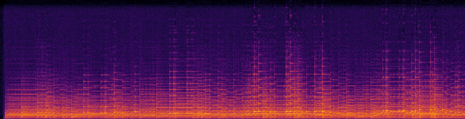
Magnitude (top) and phase (bottom) spectrums from a piano recording. X-axis is time, Y-axis is frequency. Source.
Notice that the magnitude spectrogram is easily interpretable, but phase looks essentially random. Unsurprisingly, it follows that magnitude spectrograms carry most of the perceptually important information about audio signals and so for analysis, phase can often be discarded altogether. However, phase is still quite important for generating high-quality outputs. To see what I mean, listen to the following piano piece with its original phase information and with a random phase.
Left: piano recording with original phase. Right: the same with random phase. Source.
You can still hear the melody with a random phase, but it doesn’t sound like something you’d want to come out of a generative audio model.
Generating spectrograms
If you have both magnitude and phase components for a signal, you can do an inverse STFT operation to get back to a waveform. However, given that magnitude spectrums alone offer an effective and more condensed way to model audio signals… can you just drop the phase component altogether?
As it turns out – yes this is feasible, and commonly done! The only issue is getting the result back into the time domain as a waveform. Here we have several options.
For sequence-to-sequence problems, one strategy is to use the original phase component of the input signal.
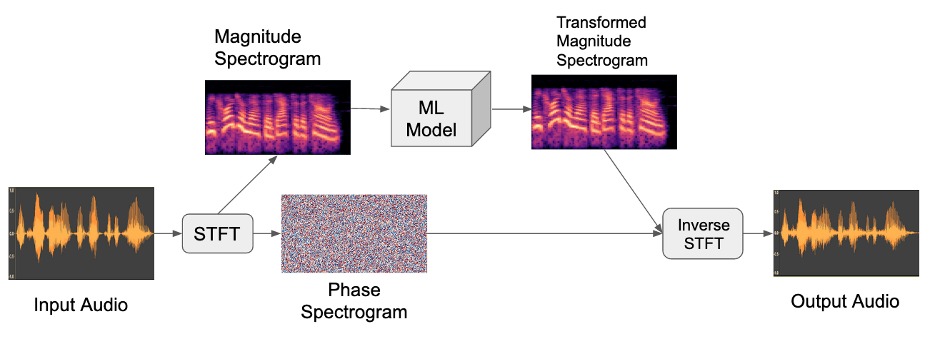
Sequence-to-sequence audio modeling in the magnitude spectral domain by re-using the original phase.
This can work, but it might not sound great for longer sequences that were drastically transformed by the model.
When that’s not feasible, another option is to come up with a phase component from scratch. This is the field of research called phase reconstruction. One time-tested approach is the Griffin-Lim algorithm, which uses the intuition that the STFT usually results in the same frequencies being activated in neighboring frames to iteratively come up with a reasonable guess for a phase.
More recently, generative models like the WaveNet[1] and WaveGlow[2] have been used as “vocoders”, or front-end components that probabilistically generate waveforms given magnitude spectrograms. You can either add these to your neural net architecture and train it all end-to-end, or you can use pretrained versions and just focus on training your custom components.
In recent years it has seemed like generative audio research was heading in the direction of always modeling the waveform domain end-to-end. However, high quality vocoders like WaveNet have enabled researchers to continue utilizing the more compact and in some cases better performing magnitude spectrograms as primary modeling domains.
With that out of the way, onto the loss functions.
L1 and L2 of waveforms
These are the bread and butter of learning objectives. If you need a reminder: L1, also known as Mean Absolute Error (MAE), involves simply aligning the two waveforms, finding the absolute difference between each pair of sample points, and averaging them. L2, or Mean Squared Error (MSE) is the exact same except you square each difference before averaging, which has the effect of penalizing larger errors and being more forgiving of smaller ones.
L1 and L2 are used all the time for audio models in the waveform domain, including many of the top music source separation approaches [3, 4, 5, 6], and are always worth a try. However, there are some potential weaknesses to be aware of.
For one, they don’t reflect natural biases in human hearing. Interestingly, we perceive certain frequencies to be louder or quieter than others, even when they played with an equal amount of energy. In the 1930’s, researchers actually measured this, resulting in the first of many “curves” that try to capture human loudness bias as a function of frequency.

If training a model for human ears, with L1/L2 you risk overweighting the importance of low frequency sounds. One way around this is to use pre-emphasis filters, which will adjust the energy levels of different frequency channels according to an equal-loudness curve, such as the one above. Librosa and SpeechPy offer this functionality.
They also fail to correlate well with human judgement of speech quality and intelligibility [7]. This makes sense from an evolutionary standpoint – humans had plenty of reasons to favor our ability to perceive speech, so we evolved neural pathways adept at doing that, which simpler metrics might not capture.
Shift Invariance
Another issue of note is that L1 and L2 in the waveform domain are not shift invariant. If your models comes up with the exact correct output, but it’s shifted just 1 millisecond too early or late, a human would consider it a perfect match but error would likely spike. This can especially manifest as phase shift invariance, where two waves have similar frequencies but out-of-sync phases, leading to a large gap in waveform distance.
This might not be a problem for you depending on your goals, or your model of choice. Recent approaches for sequence-to-sequence problems are converging on the U-Net architecture, or similar. These models have skip connections, which are more robust to shift invariance because they have access to the original input waveform late in the forward pass.
One trick for incorporating shift invariance is Dynamic Time Warping (DTW), whereby dynamic programming is used to find the minimal-cost alignment path between two time series. This means they can be considered a close match even with mutations or temporal shifts. A great example can be found in the paper “End-to-End Adversarial Text-to-Speech”[31], where DTW is used to give the model flexibility on the timing of speech utterances. Note that for loss functions, you will need to use the differentiable variant soft-DTW.
Aside from shifts, there are other transformations for which L1/L2 will unfairly penalize. When it comes to loss functions and evaluation metrics, it’s important to keep in mind which invariances you care about as a researcher.
Waveform L1/L2 make for great baselines, and it is also common to see them added to other losses.
Spectral Losses
Earlier I mentioned how magnitude spectrograms resulting from Fourier transforms offer a rich data representation, great for both analysis and generation. What I didn’t mention is that STFT is a differentiable operation! It should be unsurprising then that L1 and L2 work well as loss functions in the spectral domain, too. Sometimes you will see this referred to as spectral loss, though there are enough variations that I consider it a family of loss functions.
If your model is already working with spectrograms, then applying L1/L2 is trivial. But even if it stays in the waveform domain, both tensorflow and pytorch offer differentiable tensor versions of the STFT that you can apply during training only.
Usually the log magnitude spectrogram is used, sometimes with a small number epsilon added first, which controls the trade-off between accurately representing low energy and high energy spectral components [8].
$$ \big|\big| log(|STFT(y)| + \epsilon) - log(|STFT(\hat{y})| + \epsilon)\big|\big|_{\ell} $$ Log magnitude loss. Here \(y\) is the target signal, \(\hat{y}\) is the predicted, \(||\cdotp||_{\ell}\) is the \(\ell\) norm (like L1 or L2), and \(\epsilon\) is a small number. The absolute value around STFT is a way to discard the phase component.
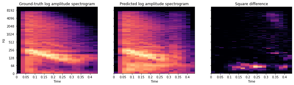
Log magnitude spectrogram of an example sound, a prediction from a model, and their squared difference.
As mentioned previously, STFT involves sliding a window across a waveform, taking Fourier transforms as you go. This hints at a couple of parameters that will effect the resulting spectrogram, and thus any downstream learning. For one, you have to choose a window size. Larger windows will be able to capture smaller frequencies, but will take up more space. You also need a hop length – it’s common to have successive windows of samples overlap each other, and hop length in relation to window size determines the extent of this overlap. In order to minimize the bias of any one choice of parameter, sometimes people use a multi-resolution spectral loss by summing the results of several runs with different window parameters.
Although logarithmic magnitude spectral losses are more common, you do sometimes see magnitude squared. In signal processing terminology, this turns amplitude into power, and so you will see this called power loss. As you can see below, a power spectrum concentrates around the strongest frequency bands, drowning out the others. It follows that power loss is great at ensuring your predictions have an accurate distribution across the frequency spectrum, in line with your target domain. For example, it could help a text-to-speech (TTS) system match the highs and lows of believable human speech [9].
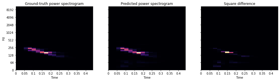
Power spectrogram of an example sound, a prediction from a model, and their squared difference.
Another related loss you might see is spectral convergence loss:
$$ \frac{\big|\big| |STFT(y)| - |STFT(\hat{y})| \big|\big|_E}{\big|\big| |STFT(\hat{y})| \big|\big|_E} $$
\(||\cdotp||_E\) above \(x\) is the Euclidean matrix norm (AKA Frobenius norm). In words: you take the Euclidean distance of the difference between two magnitude spectrograms, and normalize it by the Euclidean “length” of the original signal. Similarly to the power spectrum, since we’re squaring each error component, it highly emphasizes when any one frequency bucket prediction is way off, and is more forgiving of several frequency bucket predictions being just a little bit off. According to one paper I read [10], this can especially help in early phases of training.
Mel spectrogram loss
Earlier I mentioned how humans have natural biases in how we hear loudness at different frequencies. We also have biases in how we hear pitch. Low frequencies sound “low” to us, and higher ones sound “high”, but the relationship between frequency and perception is non-linear – a 100 Hz and 200 Hz sine wave will sound much further apart than a 10,000 Hz and 10,100 Hz wave. There have been several attempts at codifying this relationship through listening tests; the most widely used formulation is the Mel scale. Obtaining the Mel spectrogram is similar to the STFT operation, but frequency energies are placed into different buckets of equal perceived pitch difference, according to the filterbanks of the Mel scale.
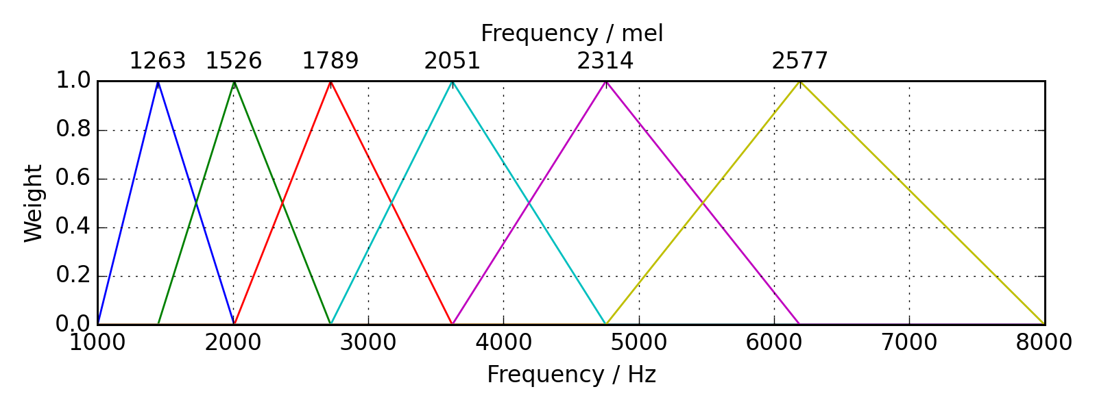
The Mel filterbank, showing windows of frequencies that are aggregated into a Mel spectrogram. Source.
Any of the previously mentioned spectral losses can also be carried out using the Mel spectrogram.
A quick side note: the Mel spectrogram is actually a common general representation for modeling audio.
Along with being a better correlate with human pitch perception, it’s also more compact
then normal spectrograms. How much so depends on how precise you make the Mel filterbanks
(e.g. the n_mels parameter in librosa), but depending on your problem, you can potentially
reduce your space footprint by an order of magnitude without sacrificing performance.
You will, however, need a specialized vocoder model if you want to get back to waveforms from a Mel spectrogram.
Spectral losses come up in many areas, but especially speech enhancement, TTS, and music synthesis.
Source Separation
Audio source separation is the problem of separating an audio signal into the components (sources)
that were mixed together to create it. One application is in music, where source
separation can be used to “demix” a song (usually into predefined categories, like bass, drums,
vocals, and other). Another application is voice separation,
which attempts to tackle the classic cocktail party problem
by isolating individual voices from a conversation, or from the background of a recording.
During model training, each predicted source is compared to a ground truth target using an objective function. While the losses covered above can work just fine, another is more common. For the following, suppose you are trying to predict the source signal \(s\), and your model comes up with an imperfect \(\hat{s}\).
SDR (Source to Distortion Ratio):
\[SDR := 10 \cdot log_{10}\frac{||s||^2}{||s - \hat{s}||^2}\]This metric is measured in decibels, where higher is better. Any mistake in the prediction will cause the denominator to grow, which will cause the overall metric to go down.
SDR is equivalent to the classic signal-to-noise ratio, so sometimes you will see it reported as SNR. However, there is a totally different SNR metric (Sources to Noise Ratio) also sometimes used to evaluate source separation results, so be careful to know which one you’re dealing with.
Scale invariance
A major downside of vanilla SDR is that it’s sensitive to the loudness of the predicted signal. If you were to scale the prediction up or down, the metric would rise or fall along a curve around some point of “ideal” scale. In the context of SDR as an evaluation metric, this means some researchers might optimize scale to achieve the highest score and others might not, leading to unfair comparisons. In the context of SDR as an objective function, I think this would lead to a slower and less-smooth learning curve.
Thankfully, some researchers surfaced the issue in 2018 and came up with a scale-invariant version of SDR where the optimal scaling factor is baked in.
SI-SDR (Scale-Invariant Source to Distortion Ratio):
\[SI-SDR := 10 \cdot log_{10}\Bigg(\frac{||\frac{\hat{s}^Ts}{||s||^2} s||^2}{||\frac{\hat{s}^Ts}{||s||^2} s - \hat{s}||^2}\Bigg)\]Again, sometimes you will see this reported as SI-SNR. At this point, I see no reason why anyone would want to use plain SDR in favor of
the scale-invariant version.
Permutation invariance
When you know the categories of sources ahead of time and your training set comes with labeled sources, you can just add the losses from each prediction. However, for problems with an unknown number of sources (called blind source separation), such as in the cocktail party problem, it’s not that simple. You need to know which predictions correspond to which ground truth targets. Further, you’ll want a one-to-one correspondence between the predictions and targets, so that you don’t end up with two predictions of the same source or not enough predicted sources. Using random assignments at every optimization step would unfairly penalize the model for a bad roll of the dice, leading to very unstable training. Rather, in these cases you should apply your loss function in a permutation invariant way. One such method is Permutation Invariant Training (PIT), wherein every combination of assignments is attempted, and the best set (lowest combined loss) is used. This incentivizes the model to settle into learning each source once, without needing to care in what order they are output.
The asteroid library offers a wrapper Python class
that makes it easy to turn any loss function into a permutation-invariant version.
Perceptual Loss
Neural networks are great at discovering features that distinguish between inputs. And it’s often easy to imagine other problems for which the same features would be helpful. For example, a facial recognition model might have a neuron that fires when presented with a horizontal line, which might be used by a higher-level neuron to decide whether the picture contains a chin. If you were then designing a person-detection model, it could probably benefit from being able to detect both chins and faces.
So how could you utilize features from a network trained to solve problem \(A\) to help train a network to solve a similar problem \(B\)? This is the research area known as transfer learning. The simplest way is to directly feed the feature values into your new network. In our example above, the person-detection network would see its normal inputs, but would also be given the neuron values from the facial detection network to work with. Another way is fine-tuning, where network \(A\) is first trained to solve problem \(A\), and then further trained to solve problem \(B\).
Neural features are not just numbers; they are connected to other neurons, that, once fully unrolled, are large differentiable functions. We should be able to utilize these function gradients without being forced to re-use the neural architecture of network \(A\) to solve problem \(B\). These are the insights that motivate perceptual loss, also known as deep feature loss. Perceptual loss was inspired by research on style transfer in computer vision.
Lets assume you have already trained an auxiliary task \(B\) (seen in the figure below in red). The basic idea is to use the features of \(B\) to compute a gradient that updates \(A\) in a way that makes audio predicted by \(A\) closer to ground-truth audio in \(B\)’s feature space. Usually in deep learning the parameters being updated during optimization are the same ones that were used to compute the gradient. However, here \(B’s\) parameters are frozen.
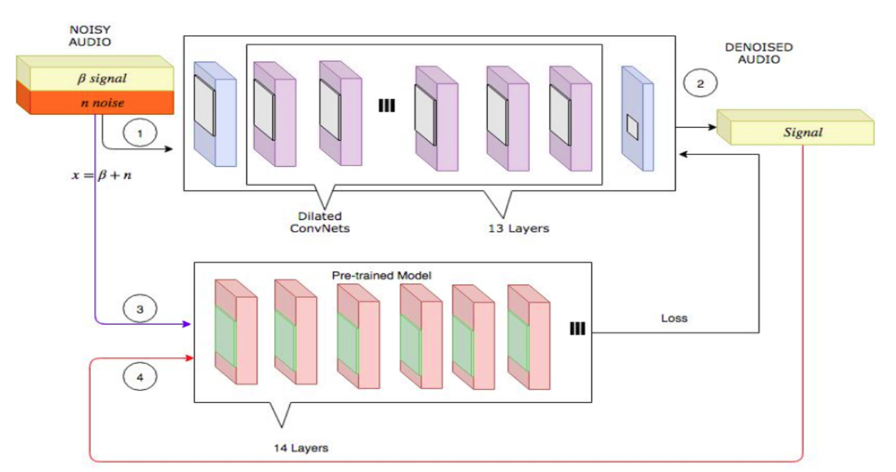
A depiction of perceptual loss learning in the audio denoising domain. First a batch
of training inputs is put through the network being optimized (top). The output is then put
through an auxiliary network (bottom), pre-trained on a similar problem. Finally, the original
batch of signals is also put through the auxiliary network, and the two activations
are compared to compute a gradient that updates the original network. Source.
The loss formula is usually something called feature reconstruction loss, where you sum the L1/L2 distances of neural activations of the auxiliary network’s first \(k\) layers. Using earlier layers favors reusable patterns over high-level features that tend to be specific to the auxiliary task.
Here are some examples from audio research:
- “Parallel wavenet: Fast high-fidelity speech synthesis”[9] – among other loss components, they include a perceptual loss term using a network trained to detect the phonemes of speech signals. They basically utilize speech-to-text features as a means of improving text-to-speech, which I find to be an interesting parrallel.
- “Voice Separation with an Unknown Number of Multiple Speakers”[11] – they attempt the cocktail party problem using perceptual loss against a networked trained on speaker identification. The intuition is that if a network is able to pick apart the nuances of different speakers’ voices, it should also provide useful features for separating voices from background audio.
- “Hierarchical Timbre-Painting and Articulation Generation”[12] – they attempt a kind of music synthesis whereby you take a source recording of some instrument playing a melody, and render it as a completely different instrument, while preserving the nuances of pitch and loudness. Their auxiliary network of choice is the pitch-detecting CREPE, with some pretty cool results here.
- “Deep Network Perceptual Losses For Speech Denoising”[13] – they utilize a deep feature loss based on speech detection as an auxiliary task, as well as one trained on the audio event detection dataset AudioSet.
Learned Perceptual Loss
In the search for a metric that highly correlates with human perception, the authors of “A Differentiable Perceptual Audio Metric Learned from Just Noticeable Differences”[14] take a unique approach.
They first crowdsource a dataset of human judgements that capture “just noticeable differences” (JND) – users are presented with two audio recordings, where one is a slightly perturbed version of the other, and asked whether they are exactly the same sounds or not. The amount of perturbation (e.g. reverb, compression, dropouts) is carefully chosen to be small enough so that the authors end up with lots of data right around the threshold of what’s barely noticeable.
They then fit a deep neural network to predict these human judgements, by minimizing binary cross-entropy. The resulting network can be used as a quality metric, and, since it is differentiable, as a learning objective (similarly to how you would use the perceptual losses above). They call their metric DPAM, available for both tensorflow and pytorch. More recently they released an improved metric called CDPAM[15], which is more robust to perturbations not used in the original JND dataset.
The released version of CDPAM is meant to be general-purpose, but their approach also seems quite adaptable. If you have particular requirements for your ideal similarity metric, or you’re working in a specialized domain with access to a pool of experts, you should be able to capture your requirements in a JND dataset and train a metric yourself.
Other
Speech Quality Metrics
If you work in speech enhancement or TTS, you may come across the metric PESQ. Originally a commercial telecomm specification, it is differentiable, but only defined up to frequencies of 8k so not ideal for learning [16]. It did inspire a newer trainable variant PMSQE[17], which looks promising.
You may also come across Short-Time Objective Intelligibility (STOI)[18], which is differentiable but usually just used as an evaluation metric.
Categorical cross entropy
You might not have expected to see a categorical loss for inherently continuous waveform data. Nonetheless, architectures like WaveNet[1] model waveform sample probabilities as discrete classes under a softmax distribution.
One benefit of quantization is that it prevents mode collapse. Sometimes models predicting continuous-valued waveforms will cut their losses by mostly just outputting the safest option between -1 and 1: zero (or near it). This is especially true earlier in the training process. By instead predicting non-ordinal classes, no such safe option exists and the model is forced into trying something.
Conclusion
During my informal survey of research from the past five years or so, I noticed some trends:
| In… | They tend to use… |
|---|---|
| Music Source Separation | L1/L2 of waveforms [3][4][5][6] |
| Speech Separation | SI-SDR [11][19][20][21] |
| Voice Conversion | L1/L2 in Mel spectral domain, adversarial losses [22][23][24] |
| Text-to-speech | L1/L2 in spectral domains, especially Mel [25][26][27][28][29][30] |
These are not endorsements, just patterns. Other areas had no clear consensus. Here are some additional tips for practitioners:
- Start with L1 in whichever domain is easiest given your model architecture, then expand your search.
- Don’t be afraid to mix several loss functions. It’s not uncommon to see three or even four components.
- Strive to use as many evaluation metrics as you can. Be especially careful if you’re using the same metric for both an objective function and evaluation, as it may leave you thinking your model is performing better than it actually is.
If you’re using pyTorch and looking to try some of these out, I recommend the auraloss library, or asteroid if you’re working on source/voice separation. Sadly I could not find anything similar for tensorflow (any readers in need of a side project?…)
There are many objective functions available for your audio models, and given the number of potential combinations, you may not be able to try them all. By being informed about their pros, cons, and prevalences, I hope you can save precious GPU hours.
References
- [1] A. Oord. WaveNet: A generative model for raw audio, 2016.
- [2] R. Prenger. WaveGlow: a Flow-based Generative Network for Speech Synthesis, 2018.
- [3] A. Défossez. Music Source Separation in the Waveform Domain, 2019.
- [4] D. Stoller. Wave-U-Net: A Multi-Scale Neural Network for End-to-End Audio Source Separation, 2018.
- [5] R. Hennequin. Spleeter: a Fast and Efficient Music Source Separation Tool with Pre-Trained Models, 2020.
- [6] N. Takahashi. D3Net: Densely connected multidilated DenseNet for music source separation, 2020.
- [7] S. Fu. MetricGAN+: An Improved Version of MetricGAN for Speech Enhancement, 2021.
- [8] A. Défossez. SING: Symbol-to-Instrument Neural Generator, 2018.
- [9] A. Oord. Parallel WaveNet: Fast High-Fidelity Speech Synthesis, 2017.
- [10] S. Arik. Fast Spectrogram Inversion using Multi-head Convolutional Neural Networks, 2018.
- [11] E. Nachmani. Voice Separation with an Unknown Number of Multiple Speakers, 2020.
- [12] M. Michelashvili. Hierarchical Timbre-Painting and Articulation Generation, 2020.
- [13] M. Saddler. Deep Network Perceptual Losses For Speech Denoising, 2020.
- [14] P. Manocha. A Differentiable Perceptual Audio Metric Learned from Just Noticeable Differences, 2020.
- [15] P. Manocha. CDPAM: Contrastive learning for perceptual audio similarity, 2021.
- [16] POLQA Vs PESQ: Objective quality scoring explained.
- [17] J. Martín-Doñas. A Deep Learning Loss Function based on the Perceptual Evaluation of the Speech Quality, 2019.
- [18] C. Taal. A short-time objective intelligibility measure for time-frequency weighted noisy speech, 2010.
- [19] Y. Luo. Conv-TasNet: Surpassing Ideal Time-Frequency Magnitude Masking for Speech Separation, 2019.
- [20] C. Subakan. Attention is All You Need in Speech Separation, 2020.
- [21] M. Pariente. Filterbank design for end-to-end speech separation, 2019.
- [22] H. Kameoka. StarGAN-VC: Non-parallel many-to-many voice conversion with star generative adversarial networks, 2018.
- [23] S. Wang. NoiseVC: Towards High Quality Zero-Shot Voice Conversion, 2021.
- [24] J. Zhang. Sequence-to-Sequence Acoustic Modeling for Voice Conversion, 2018.
- [25] Y. Wang. Tacotron: Towards End-to-End Speech Synthesis, 2017.
- [26] J. Shen. Natural TTS Synthesis by Conditioning WaveNet on Mel Spectrogram Predictions, 2017.
- [27] Y. Jia. Transfer Learning from Speaker Verification to Multispeaker Text-To-Speech Synthesis, 2018.
- [28] A. Gritsenko. A Spectral Energy Distance for Parallel Speech Synthesis, 2020.
- [29] X. Wang. Neural source-filter-based waveform model for statistical parametric speech synthesis, 2018.
- [30] W. Ping. Deep Voice 3: Scaling Text-to-Speech with Convolutional Sequence Learning, 2017.
- [31] J. Donahue. End-to-End Adversarial Text-to-Speech, 2021.